Suppose that a program takes T_c time to execute on c cores. Thus, the serial version of the program would take T₁ time.

The speedup of the program on c cores is then expressed by the equation:

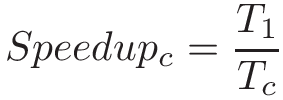
If a serial program takes 60 seconds to execute, while its parallel version takes 30 seconds on 2 cores, the corresponding speedup is 2. Likewise if that program takes 15 seconds on 4 cores, the speedup is 4. In an ideal scenario, a program running on n cores with n total threads has a speedup of n.

If the speedup of a program is greater than 1, it indicates that the parallelization yielded some improvement. If the speedup is less than 1, then the parallel solution is in fact slower than the serial solution. It is possible for a program to have a speedup greater than n (for example, as a side effect of additional caches reducing accesses to memory). Such cases are referred to as superlinear speedup.

Speedup doesn’t factor in the number of cores — it is simply the ratio of the serial time to the parallel time. For example, if a serial program takes 60 seconds, but a parallel program takes 30 seconds on four cores, it still gets a speedup of 2. However, that metric doesn’t capture the fact that it ran on four cores.

To measure the speedup per core, use efficiency:

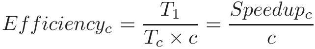
Efficiency typically varies from 0 to 1. An efficiency of 1 indicates that the cores are being used perfectly. If efficiency is close to 0, then there is little to no benefit to parallelism, as the additional cores do not improve performance. If efficiency is greater than 1, it indicates superlinear speedup.

Let’s revisit the previous example, in which a serial program takes 60 seconds. If the parallel version takes 30 seconds on two cores, then its efficiency is 1 (or 100%). If instead the program takes 30 seconds on four cores, then the efficiency drops to 0.5 (or 50%).

In an ideal world, speedup is linear. For each additional compute unit, a parallel program should achieve a commensurate amount of speedup. However, this scenario rarely occurs in the real world. Most programs contain a necessarily serial component that exists due to inherent dependencies in the code. The longest set of dependencies in a program is referred to as its critical path. Reducing the length of a program’s critical path is an important first step in its parallelization. Thread synchronization points and (for programs running on multiple compute nodes) communication overhead between processes are other components in the code that can limit a program’s parallel performance.

Consider the parallelization of the countElems function of the CountSort algorithm from earlier in this chapter. In an ideal world, we would expect the speedup of the program to be linear with respect to the number of cores. However, let’s measure its runtime (in this case, running on a quad-core system with eight logical threads):

Table 1 shows the speedup and efficiency for these multithreaded executions:

While we have 84% efficiency with two cores, the core efficiency falls to 39% with eight cores. Notice that the ideal speedup of 8 was not met. One reason for this is that the overhead of assigning work to threads and the serial update to the counts array starts dominating performance at higher numbers of threads. Second, resource contention by the eight threads (remember this is a quad-core processor) reduces core efficiency.

In 1967, Gene Amdahl, a leading computer architect at IBM, predicted that the maximum speedup that a computer program can achieve is limited by the size of its necessarily serial component (now referred to as Amdahl’s Law). More generally, Amdahl’s Law states that for every program, there is a component that can be sped up (i.e., the fraction of a program that can be optimized or parallelized, P), and a component that cannot be sped up (i.e., the fraction of a program that is inherently serial, or S). Even if the time needed to execute the optimizable or parallelizable component P is reduced to zero, the serial component S will exist, and will come to eventually dominate performance. Since S and P are fractions, note that S + P = 1.

Consider a program that executes on one core in time T₁. Then, the fraction of the program execution that is necessarily serial takes S × T₁ time to run, and the parallelizable fraction of program execution (P = 1 - S) takes P × T₁ to run.

When the program executes on c cores, the serial fraction of the code still takes S × T₁ time to run (all other conditions being equal), but the parallelizable fraction can be divided into c cores. Thus, the maximum improvement for the parallel processor with c cores to run the same job is:

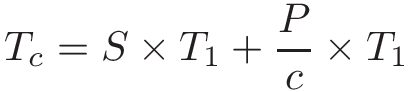
As c increases, the execution time on the parallel processor becomes dominated by the serial fraction of the program.

To understand the impact of Amdahl’s law, consider a program that is 90% parallelizable and executes in 10 seconds on 1 core. In our equation, the parallelizable component (P) is 0.9, while the serial component (S) is 0.1. Table 2 depicts the corresponding total time on c cores (T_c) according to Amdahl’s Law, and the associated speedup.

Observe that, over time, the serial component of the program begins to dominate, and the effect of adding more and more cores seems to have little to no effect.

A more formal way to look at this requires incorporating Amdahl’s calculation for T_c into the equation for speedup:

Taking the limit of this equation shows that as the number of cores (c) approaches infinity, speedup approaches 1/S. In the example shown in Table 2, speedup approaches 1/0.1, or 10.

As another example, consider a program where P = 0.99. In other words, 99% of the program is parallelizable. As c approaches infinity, the serial time starts to dominate the performance (in this example, S = 0.01). Thus, speedup approaches 1/0.01 or 100. In other words, even with a million cores, the maximum speedup achievable by this program is only 100.